Linear Programming
A linear programming problem is an optimization problem where:
- The objective function F : X \to R is linear , where X is the feasible region.
- The feasible region has linear constraints.
A solution \underline{x}^* \in R^n is said to be optimal if f(\underline{x}^*) beats f(\underline{x}), \forall \underline{x} \in X.
Traditional representations:
General form
\begin{align*} min \quad &z = c_1 x_1 + \dots + c_nx_n \\ & a_{11} + \dots + a_{1n}x_n (\geq,=,\leq) b_1\\ &\vdots\\ & a_{m1}x_1+\dots + a_{mn}x_n (\geq,=,\leq) b_m\\ &x_1,\dots,x_n \geq 0 \end{align*}
Matrix form
\begin{align*} min \quad &z = \underline{c}^T \underline{x} \\ s.t.\quad & A\underline{x} \geq \underline{b} \\ &\underline{x} \geq 0 \end{align*} min \quad z = [c_1 \dots c_n] \begin{bmatrix} x_1 \\ \vdots\\ x_n \end{bmatrix} s.t. \quad \begin{bmatrix} a_{11} & \dots & a_{1n} \\ \vdots & & \vdots\\ a_{m1} & \dots & a_{mn} \end{bmatrix} \begin{bmatrix} x_1 \\ \vdots \\ x_n \end{bmatrix} \geq \begin{bmatrix} b_1 \\ \vdots \\ b_m \end{bmatrix}
\begin{bmatrix} x_1 \\ \vdots \\ x_n \end{bmatrix} \geq \underline{0}
General Assumptions
Consequences of the linearity:
- Proportionality: Contribution of each variable = constant \times variable , we often refer to these constants as parameters.
- Additivity: Contribution of all variable = sum of single contributions : f(x + y + z) = f(x) + f(y) + f(z)
In these types of problems variables can take any rational values.
Parameters are constants.
Example:
Suppose that we want to maximize how much we gain from the selling of 5 products ( suppose that we sell and produce the products in grams) , the profits/g of each one of them are respectively: 2, 3, 4, 5, 6; the cost of production of each one of them is: 3, 6, 7, 9, 10; no more than 400g must be produced and the total production cost must be lower than 3000. We shall model this problem like this:
Traditional modelling
\begin{align*} max \quad & 2\mathscr{x}_1 + 3\mathscr{x}_2 + 4\mathscr{x}_3 + 5\mathscr{x}_4 + 6\mathscr{x}_5 \\ s.t. \quad & 3\mathscr{x}_1 + 6\mathscr{x}_2 + 7\mathscr{x}_3 + 9\mathscr{x}_4 + 10\mathscr{x}_5 \leq 3000 \quad (1)\\ & \mathscr{x}_1 + \mathscr{x}_2 + \mathscr{x}_3 + \mathscr{x}_4 + \mathscr{x}_5 \leq 400\quad(2)\\ & \mathscr{x}_i \geq 0, \forall i \in {1,2,3,4,5} \end{align*}
- Maximum production cost
- Maximum quantity produced
Using python’s mip library
import mip
from mip import CONTINUOUS

# these are our parameters
I = [0, 1, 2, 3, 4] # Products
P = [2, 3, 4, 5, 6] # Profits
C = [3, 6, 7, 9, 10] # Costs
Cmax = 3000 # Max total cost
Qmax = 400 # Max total amount of product


model=mip.Model()
x = [model.add_var(name=f"x_{i+1}", lb=0 ,var_type=CONTINUOUS) for i in I]

# Objective function
model.objective = mip.maximize(mip.xsum(P[i] * x[i] for i in I))

# Constraints

# Maximum production cost
model.add_constr(mip.xsum(x[i]*C[i] for i in I) <= 3000)

# Maximum quantity produced
model.add_constr(mip.xsum(x[i] for i in I)<= 400)

model.optimize()
for i in model.vars:
    print(i.name,i.x)
Geometry of linear Programming
A couple of definitions:
- A hyperplane defined as H = {\,\underline{x} \in R^n : \underline{a}^T \underline{x} = b\,} is a flat surface that generalize a two-dimensional plane (in our case where b \ne 0 is said to be an affine hyperplane).
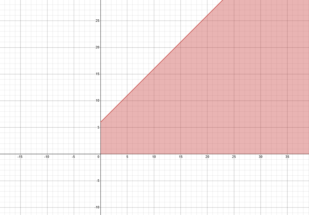
- An affine half-space defined as H^- = {\,\underline{x} \in R^n:\underline{a}^T \underline{x} \leq b \,} is the region that lies “below” or “above” an affine hyperplane.
Each inequality constraint defines an affine half-space in the variable space.
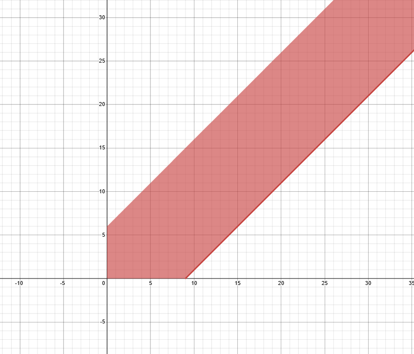
The feasible region of a linear programming problem is the intersection of a finite number of half-spaces (constraints). Said feasible region is a polyhedron.
Hyperplane (affine)
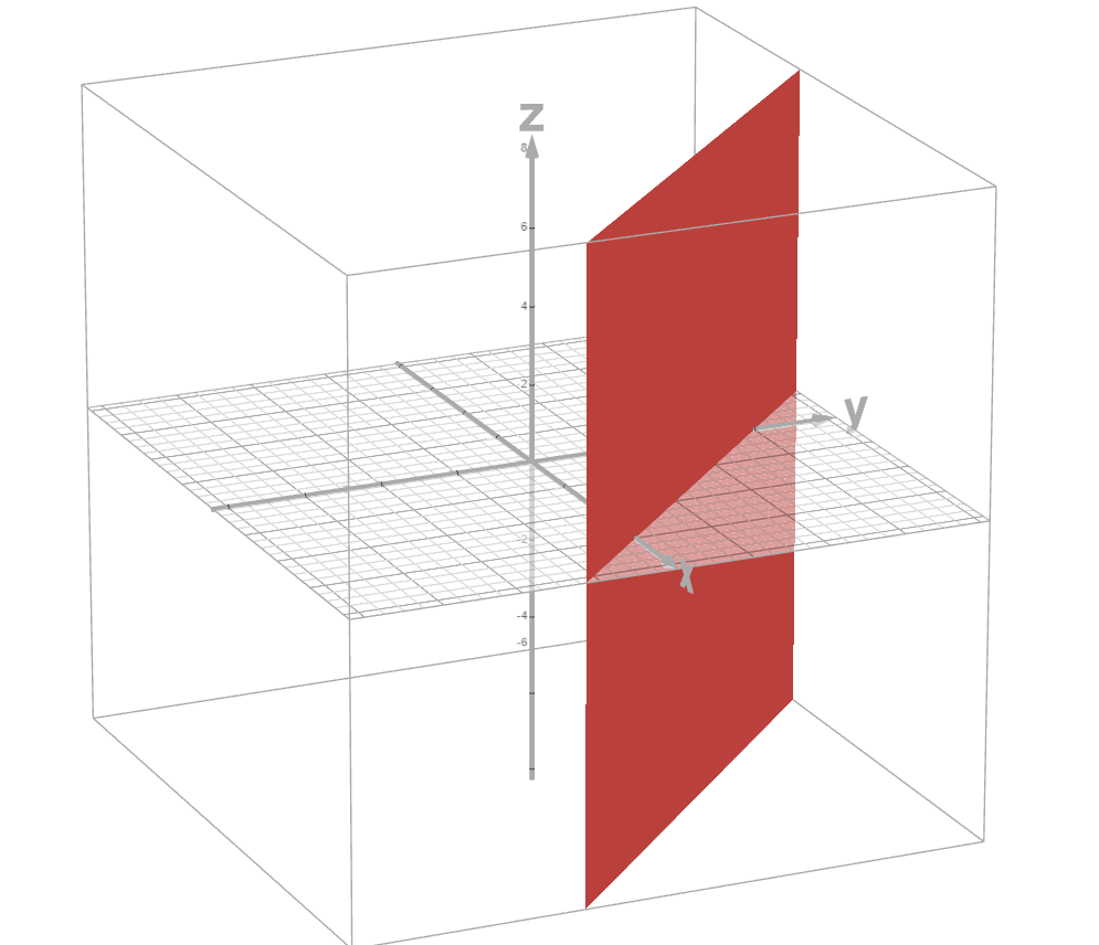
Affine half-space
Polyhedron
Convex subsets
A subset S \subseteq R^n is convex if for each pair of points \underline{x}_1,\underline{x}_2 \in S the segment defined by them is the defined by all the convex combinations of the two points: [\underline{x}_1,\underline{x}_2] = {\:\underline{p} \in R^n : \underline{x} = \alpha\underline{x}_1 + (1 - \alpha)\underline{x}_2 \, \land \alpha \in [0,1]\:}
Meaning that the subset contains the whole segment connecting the two points.
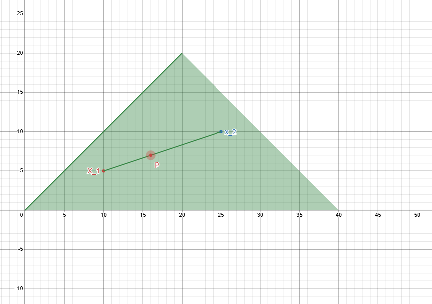
A polyhedron is a convex set of R^n \implies The feasible region of a LP is a convex set of R^n
Vertices
A vertex of a polyhedron P is a point which cannot be expressed as a convex combination of two other dinstinct points of P.
Given a point \underline{x} and a pair of points (\underline{y}_1,\underline{y}_2)
\underline{x} is a vertex \iff \:\underline{x} = \alpha\underline{y}_1 + (1 - \alpha)\underline{y}_2 \, \land \alpha \in [0,1]\: \land (\underline{x}= \underline{y}_1 \lor \underline{x}= \underline{y}_2)
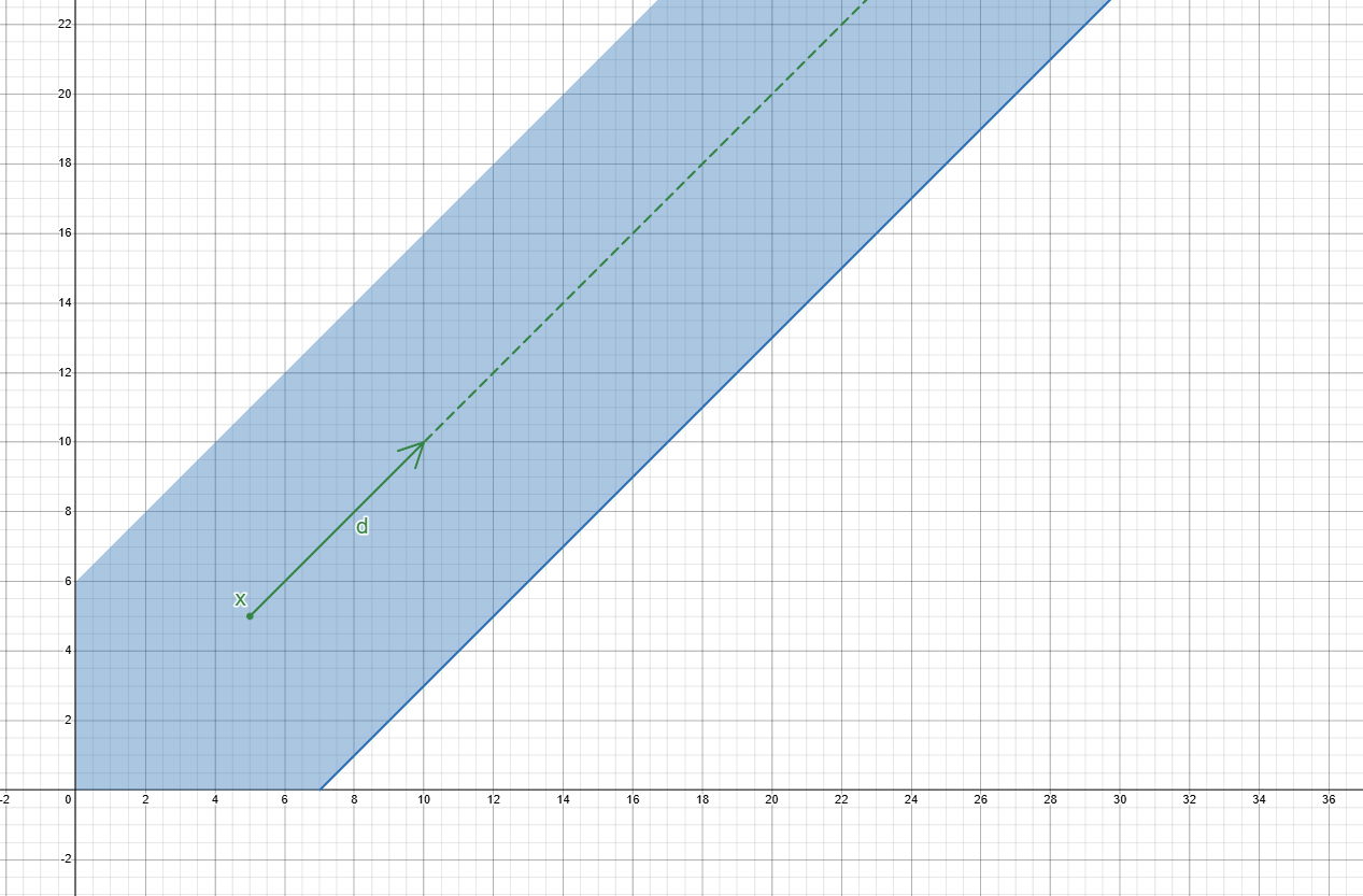
Unbounded feasible direction of polyhedron
An unbounded feasible direction d of a polyhedron P is a nonzero vector such that ,from a point \underline{x} \in P, all points of the form \underline{x} + \lambda d \: with \lambda > 0 also belongs to P. The set of such points is often called the ray of d through \underline{x}.
Polytopes
A polytope is a bounded polyhedron , hence the only unbounded feasible direction is d = 0 (so in a sense it does not have any)

Representation of polyhedra - Weyl-Minkowsky Theorem
Every point \underline{x} of a
polyhedron P can be expressed as a convex combination
of its vertices \underline{x}^1, \dots,
\underline{x}^k plus (if needed) an unbounded feasible
direction of P:
\underline{x} = \alpha_1\underline{x}_1 + \dots + \alpha_k
\underline{x}_k + \underline{d}
where \quad\sum_{i=1}^{k} \alpha_i = 1
,\:\alpha_i \geq 0 , \forall i \in { 1 \dots k}
“The
multipliers are positive and theirs sum must be equal to 1”
Standard form of LPs
Transformations rules
max \quad \underline{c}^T \underline{x} \implies -min \:(-\underline{c}^T \underline{x})
\underline{a}^T \underline{x} \leq b \implies \begin{cases} \underline{a}^T\underline{x} + s = b \\ s \geq 0 \end{cases}\quad where s is a slack variable.
\underline{a}^T \underline{x} \geq b \implies \begin{cases} \underline{a}^T\underline{x} - s = b \\ s \geq 0 \end{cases}\quad where s is a surplus variable.
x_j unrestricted sign \begin{cases} x_j = {x_j}^+\,-\,{x_j}^- \\ {x_j}^+\, , \, x_j^- \geq 0 \end{cases}\quad
After substituting x_j with {x_j}^+\,-\,{x_j}^- , we delete x_j from the problem.
Standard form
An LP is said to be in standard form if this is its appearance: \begin{align*} min \quad & z=\underline{c}^T\underline{x} \\ s.t. \quad & A\underline{x} = \underline{b} \\ & \underline{x} \geq \underline{0} \end{align*}
Example:
Let’s put the following LP in standard form:
\begin{align*} max \quad & 2\mathscr{x}_1 + 3\mathscr{x}_2 + 4\mathscr{x}_3 + 5\mathscr{x}_4 + 6\mathscr{x}_5 \\ s.t. \quad & 3\mathscr{x}_1 + 6\mathscr{x}_2 + 7\mathscr{x}_3 + 9\mathscr{x}_4 + 10\mathscr{x}_5 \leq 3000 \quad \\ & \mathscr{x}_1 + \mathscr{x}_2 + \mathscr{x}_3 + \mathscr{x}_4 + \mathscr{x}_5 \leq 400\quad\\ & \mathscr{x}_i \geq 0, \forall i \in {1,2,3,4} \: , \mathscr{x}_5 \in R \end{align*}
- From maximization to minimization \begin{align*} min \quad & -2\mathscr{x}_1 - 3\mathscr{x}_2 - 4\mathscr{x}_3 - 5\mathscr{x}_4 - 6\mathscr{x}_5 \\ s.t. \quad & 3\mathscr{x}_1 + 6\mathscr{x}_2 + 7\mathscr{x}_3 + 9\mathscr{x}_4 + 10\mathscr{x}_5 \leq 3000 \quad \\ & \mathscr{x}_1 + \mathscr{x}_2 + \mathscr{x}_3 + \mathscr{x}_4 + \mathscr{x}_5 \leq 400\quad\\ & \mathscr{x}_i \geq 0, \forall i \in {1,2,3,4} \: , \mathscr{x}_5 \in R \end{align*}
- From inequality to equalities by adding slack variables \begin{align*} min \quad & -2\mathscr{x}_1 - 3\mathscr{x}_2 - 4\mathscr{x}_3 - 5\mathscr{x}_4 - 6\mathscr{x}_5 \\ s.t. \quad & 3\mathscr{x}_1 + 6\mathscr{x}_2 + 7\mathscr{x}_3 + 9\mathscr{x}_4 + 10\mathscr{x}_5 + S_1 = 3000 \quad \\ & \mathscr{x}_1 + \mathscr{x}_2 + \mathscr{x}_3 + \mathscr{x}_4 + \mathscr{x}_5 + S_2 = 400\quad\\ & \mathscr{x}_i \geq 0, \forall i \in {1,2,3,4} \: , \mathscr{x}_5 \in R \\ & S_1, S_2 \geq 0 \end{align*}
- Substituting unrestricted sign variables \begin{align*} min \quad & -2\mathscr{x}_1 - 3\mathscr{x}_2 - 4\mathscr{x}_3 - 5\mathscr{x}_4 - 6\mathscr{x}_5 \\ s.t. \quad & 3\mathscr{x}_1 + 6\mathscr{x}_2 + 7\mathscr{x}_3 + 9\mathscr{x}_4 + 10\mathscr{x}_5 + S_1 = 3000 \quad \\ & \mathscr{x}_1 + \mathscr{x}_2 + \mathscr{x}_3 + \mathscr{x}_4 + \mathscr{x}_5^+ - \mathscr{x}_5^- + S_2 = 400\quad\\ & \mathscr{x}_i \geq 0, \forall i \in {1,2,3,4} \: \\ & \mathscr{x}_5^+ , \mathscr{x}_5^- \geq 0 \\ & S_1, S_2 \geq 0 \end{align*} The problem is now in standard form.
Fundamental Theorem of Linear Programming
Consider a minimization problem in standard form where the constraints define a non-empty feasible area (polyhedron) P. Then either:
The value of the objective function is unbounded below on P.
Exists at least one optimal vertex.
Proof
Case 1:
P has an unbounded feasible direction \underline{d} such that \underline{c}^T\underline{d}<0 ,this means that proceeding in that direction will make the value smaller and smaller and the objective value tends to -\infty.
Case 2:
P has no unbounded feasible direction such that along that path the value keeps getting smaller. As we saw any point of the feasible region can be expressed as a convex combination of its vertices plus the unbounded direction, so for any \underline{x} \in P we have \underline{d} or \underline{c}^T \underline{d} \geq 0 (either the value along that direction gets bigger or that direction is \underline{0}) so:
\underline{c}^T\underline{x} = \underline{c}^T ( \sum_{i=1}^{k}{\alpha_i\underline{x}^i + \underline{d}}) =\sum_{i=1}^{k}{\alpha_i\underline{c}^T\underline{x}^i +\underline{c}^T\underline{d}} \geq min_{i=1.\dots,k}{(\underline{c}^T\underline{x}^i)}
Put in words this tells us that the objective value of any point inside the feasible region (\underline{c}^T (\sum_{i=1}^{k}{\alpha_i\underline{x}^i + \underline{d}})) will be bigger the minimum value that the objective function has in one of its vertices (the optimal vertex) : min_{i=1.\dots,k}{(\underline{c}^T\underline{x}^i)}.
This also foreshadow that the solution of any minimization problem lies in one of its vertices ( if the solution is unique)
This would likely become more clear when we see how to solve LP problems graphically.
Types of LPs
- Unique optimal solution.
- Multiple(infinite) optimal solutions.
- Unbounded LP: Unbounded polyhedron and unlimited objective function value.
- Empty polyhedron: no feasible solutions.
Solving LPs Graphically
We would like to solve this problem:
\begin{align*} max &\quad x_1+3x_2 \\ s.t. &\quad -x_1+x_2 \geq-2\\ &\quad 2x_1+x_2 \leq 10 \\ &\quad -x_1+3x_2 \leq 9 \\ &\quad x_1,x_2 \geq 0 \end{align*}
This is our feasible region (x = x_1 ; y = x_2):
Lets analyze the objective function: z=x_1+3x_2 Lets compute its gradient: \nabla z= [ 1 \quad 3]^T
This tells us where to go if we want our value to increase, since we are solving an LP this direction will always be the same.
Let’s take a level curve from our objective function by assigning z
to some constant c:
c = x_1+3x_2
Starting from 0 we see that by increasing the value of c the
level curve follows the direction of the gradient: 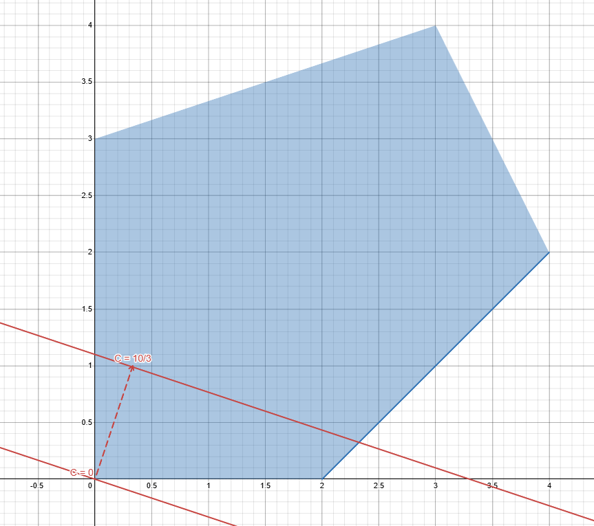
If we follow that direction we would see that it leads us to the vertex [3 \:,\: 4]^T since it the last meeting point it will give us the maximum value of the objective function:
z = 1 \times 3 + 3 \times 4 = 15
This graphical method is pretty easy to use , but it is feasible only for problems with less than 2 variables. To solve bigger problems we must find a better method.
MIP implementation:
import mip
from mip import CONTINUOUS

model = mip.Model()
# variable definition
x = [model.add_var(name = f"x_{1}", lb =0 ,var_type=CONTINUOUS), model.add_var(name = f"x_{2}", lb =0 ,var_type=CONTINUOUS)]
# objective function
model.objective = mip.maximize(x[0]+3*x[1])
# constraints
model.add_constr(-x[0]+x[1] >= -2)
model.add_constr(2*x[0]+x[1] <= 10)
model.add_constr(-x[0]+3*x[1] <= 9)

model.optimize()
for i in model.vars:
    print(i.name,i.x)
Basic feasible solutions and vertices of polyhedra
The geometrical definition of vertex cannot be exploited algorithmically because even though LPs can be viewed as combinatorial problems, and you can theoretically examine only the vertices and keep the best, the number of vertices is often exponential, so this route is not feasible.
We need algebraic characterization
Consider a polyhedron (feasible region) P = {\underline{x} \in R^n : A \underline{x} = \underline{b} , \underline{x} \geq}
Assumption: A \in R^{m\times n} (n variables and m constraints) is such that m\leq n of rank m (There are no redundant constraints)
- If m=n , there is a unique solution for A\underline{x} = \underline{b}
- If m<n , there are \infty solutions for A\underline{x} = \underline{b} . The system has n-m degrees of freedom( the number of variables that can freely change while still satisfying the constraints), n-m variables can be fixed arbitrarily and by fixing them to 0 we get a vertex.
A basis of a matrix “A” is a subset of its columns “m” that are linearly independent and form an m\timesm non-singular(invertible) matrix B. We can separate A like this:
A=[\overbrace{B}^{m} \: |\overbrace{N}^{n-m}]
Similarly to “A” we can also separate the variables in basic (“inside” of B) and non-basic (“inside” of N) , like so: \underline{x}=[\:\underline{x}_B^T\quad|\quad\underline{x}_N^T\:]\quad (1)
By substituting (1) into our system: A\underline{x} = \underline{b}; we can rewrite it as: B\underline{x}_B+N\underline{x}_n = \underline{b}
Thanks to the non-singularity of B we can describe the set of basic variables using the non-basic ones: \underline{x}_B=B^{-1}b-B^{-1}N\underline{x}_N
So lets put things together:
- A basic solution is a solution obtained by setting \underline{x}_N = \underline{0} (it’s basic because there are no non-basic variables DUH), with this our definition of basic variables becomes: \underline{x}_B = B^{-1}b
- A basic solution with \underline{x}_B \geq 0 is a basic feasible solution (the problem is in standard form, the variables are positive).
Wait , we said that by fixing n-m variables to 0 we get a vertex , but later we saw that a basic solution is obtained by setting to 0 all the non-basic variables which are also n-m, wonder what that could mean…
Not surprsingly:
vertex\quad \iff \quad basic\:feasible\:solution
Number of basic feasible solutions: At least \binom{n}{m} (from the fundamental theorem looking at LPs as combinatorial problems)
Simplex method

We discussed the need for a method that would work even for bigger problems, this method is the way to go, but before talking about it, we need to discuss a few things.
Active constraints
Let’s take a feasible region:
defined by these constraints: \begin{align*} &\quad x_1-x_2 \leq 2\\ &\quad 2x_1+x_2 \leq 10 \\ &\quad -x_1+3x_2 \leq 9 \\ &\quad x_1,x_2 \geq 0 \end{align*}
Let’s put them in standard form by adding slack variables S_1, S_2, S_3:
\begin{align*} &\quad x_1-x_2 + S_1 = 2\\ &\quad 2x_1+x_2+ S_2 = 10 \\ &\quad -x_1+3x_2 + S_3 = 9 \\ &\quad x_1,x_2,S_1,S_2,S_3 \geq 0 \end{align*}
If we decide to assign 0 to one of the slack variables,the original constraint becomes an equality, meaning that the variables will “be moving” on the “side” that the constraint describe.
By doing so we say that we activate the constraint.
In other words:
If an assignment of the variables results in a point that lies on one of the borders of the feasible region , the constraint that is responsible for that border is labelled as active.
Moving from a vertex to another
When we talked about the LP Fundamental theorem we saw how enumerating all the vertices and keeping only the best, is not a good strategy. So instead of trying to find all of them, we’ll work on how to find one by “moving” from a neighboring vertex that we already know.
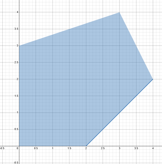
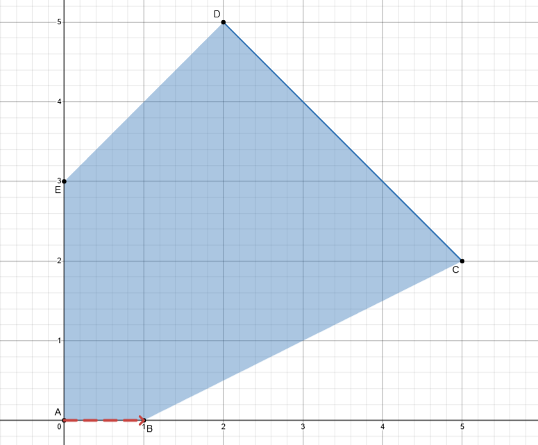
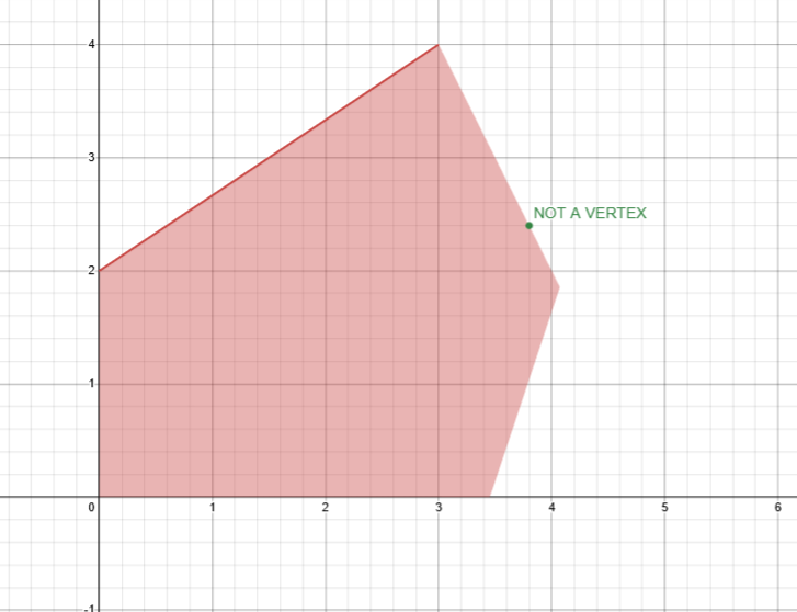
Let’s take a feasible region:
Defined by these constraints: \begin{align*} &\quad x_1+x_2 \leq 7\\ &\quad -x_1+x_2 \leq 3 \\ &\quad x_1-2x_2 \leq 1 \\ &\quad x_1,x_2 \geq 0 \end{align*}
Put in standard form:
\begin{align*} &\quad x_1+x_2+S_1 = 7 \quad (1)\\ &\quad -x_1+x_2+S_2 = 3 \quad (2)\\ &\quad x_1-2x_2+S_3 = 1 \quad (3)\\ &\quad x_1,x_2,S_1,S_2,S_3 \geq 0 \end{align*}
Our matrix A is : A= \begin{bmatrix} 1 & 1 & 1 & 0 & 0 \\ -1 & 1 & 0 & 1 &0 \\ 1 & -2 & 0 & 0 & 1 \end{bmatrix}
we have m = 3 and n = 5 so we have 2 degrees of freedom.
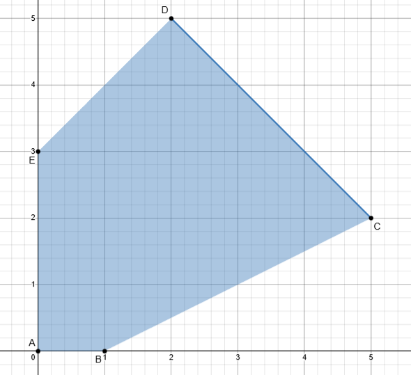
Let’s pick a starting point, we choose the vertex “A” since we just need to take out the first two columns of the matrix to find it (remember that since we are talking about vertexes the variable that are non-basic are set to 0 , and since all of Ss variables are basic none of them 0 meaning no constraints is active).
Our matrix is partitioned this way:
B= \begin{bmatrix} 1 & 0 & 0 \\ 0 & 1 &0 \\ 0 & 0 & 1 \end{bmatrix}\quad N=\begin{bmatrix} 1 & 1 \\ -1 & 1 \\ 1 & -2 \end{bmatrix}
Now lets say that we want to move from vertex A to vertex B :
How should we change our basis to achieve the goal?
We must activate the constraints whose interception defines the wanted vertex, in our case the constraint (3), so we activate it by dropping the column [0,\:0,\:1]^T from B and adding [1,\:-1,\:1]^T (we need x_2 also to be 0 so we keep it non-basic by not choosing the other column).
Our partition is now:
B= \begin{bmatrix} 1 &1 & 0 \\ -1& 0 & 1 \\ 1 &0 & 0 \end{bmatrix}\quad N=\begin{bmatrix} 1 & 0 \\ 1 & 0 \\ -2 & 1 \end{bmatrix}
And we moved to vertex B.
What if we wanted to move from B to C?
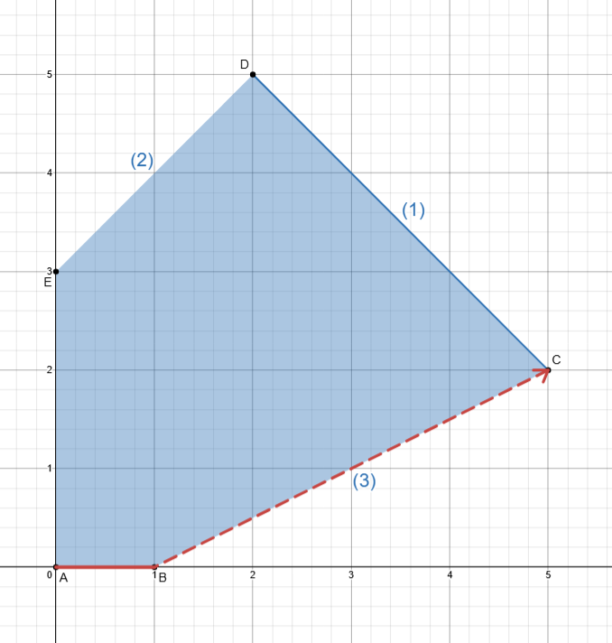
We need to activate constraint (1) since C is the meeting point of (1) and (3) so we kick S_1 out :
B= \begin{bmatrix} 1 &1 & 0 \\ -1& 1 & 1 \\ 1 &-2 & 0 \end{bmatrix}\quad N=\begin{bmatrix} 1 & 0 \\ 0 & 0 \\ 0& 1 \end{bmatrix}
We are now in vertex C.
Now that we saw how to move to neighboring vertex , we need to find a good way to determine which vertex it would be better to move to.
Reduced costs
We have an LP in standard form: \begin{align*} min\quad & z=\underline{c}^T\underline{x}\\ & A\underline{x} = \underline{b} \end{align*} Let’s now expand the objective function by making explicit the basic and non-basic parts: z = [\:\underline{c}_B^T \quad \underline{c}_N^T\:] \begin{bmatrix} \underline{x}_B \\ \underline{x}_N \end{bmatrix} \quad(1)
We previously saw how to express basic variables in terms of non-basic ones , like so (with B and N being partitions of A): \underline{x}_B=B^{-1}b-B^{-1}N\underline{x}_N \quad(2)
So we can rewrite (1) using (2) as:
z=[\:\underline{c}_B^T \quad \underline{c}_N^T\:] \begin{bmatrix} B^{-1}b-B^{-1}N\underline{x}_N \\ \underline{x}_N \end{bmatrix} \quad
That translates into: z = \underline{c}_B^T B^{-1} b-c_B^TB^{-1} N \underline{x}_N+c_N^T\underline{x}_N
Let’s group by \underline{x}_N: z = \underbrace{\underline{c}_B^T B^{-1} b}_{V}+\underline{x}_N(\underbrace{c_N^T-c_B^TB^{-1}N}_R)
The first part of the formula (V) is the value of the objective function when we are in a basic feasible solution (vertex) since \underline{x}_N is \underline{0}.
The second part of the formula (R) are the reduced costs(of then non-basic variables), but before giving you the definition let’s try to understand what are the reduced cost.
Definition walkthrough
Let’s start from our formula:
\underline{\overline{c}}_N^T = c_N^T-c_B^TB^{-1}N
The c_N^T part doesn’t tell us much ,it just is the contribution of the non-basic variables in the objective function. The c_B^TB^{-1}N part on the other hand is where the things start to get interesting.
What is B^{-1}N?
Let’s suppose that we have the following constraint: x_1 +4 x_2 + 2 x_3 + x_4 = 24
And we have these assignments: \underline{x}^T = [\:1\quad 2\quad 6 \quad3\:]
If we decided to change the value of one of the variables, how the others should adjust themselves in order to still satisfy the constraint?
This is exactly what B^{-1}N tells us.
Let’s crunch some numbers:
We have this LP:
\begin{align*} min\quad &x_1+2 x_2+3x_3+x_4\\ s.t. \quad &x_1+2x_2+x_3 = 5\\ &x_2+x_3+x_4 = 3\\ & x_1,x_2,x_3,x_4 \geq 0 \end{align*} We decide to start from a vertex by choosing x_1 and x_4 as basic variables, so we partition the matrix this way: B= \begin{bmatrix} 1 & 0 \\ 0& 1 \end{bmatrix}\quad N=\begin{bmatrix} 2 & 1 \\ 1 & 1 \end{bmatrix}
Our current assignment is: \underline{x}^T=[\:5\quad0\quad 0 \quad3\:] or
\underline{x}_B^T=[\:5\quad3\:]\quad \quad \underline{x}_N^T=[\: 0 \quad 0 \:]
The objective value is: 5 + 0 + 0 + 3 = 8 What if we increased x_2 by 1?
Let’s compute B^{-1}N: B^{-1}N=\begin{bmatrix} 2 & 1 \\ 1 & 1 \end{bmatrix} This tells us that by increasing x_2 by 1 the value of x_1 must change by a factor of 2 and x_4 by a factor of 1 (the first column), lets see it algebraically:
We know that:
\underline{x}_B=B^{-1}b-B^{-1}N\underline{x}_N
Which holds regardless whether we are in a vertex or not, we are just expressing two variables in function of the other two.
So let’s compute the new values of x_1 and x_4:
\underline{x}_B=\begin{bmatrix} 5\\ 3\end{bmatrix}-\begin{bmatrix} 2 & 1 \\ 1 & 1 \end{bmatrix}\begin{bmatrix} 1\\ 0\end{bmatrix} = \begin{bmatrix} 3\\ 2\end{bmatrix} Where [1\quad 0]^T is the new assignment of x_2.
The constraints hold:
\begin{align*} & 3 +2\times 1+0 = 5\\ &1+0+2 = 3\\ \end{align*}
The new value of the objective is:
3+2\times1+0+2 = 7
Let’s use the formula given by our previous definition:
\underline{\overline{c}}_N^T = c_N^T-c_B^TB^{-1}N
Substituting: \begin{align*} \underline{\overline{c}}_N^T &= [\:2\quad3\:] - [\:1\quad1\:]\begin{bmatrix} 2 & 1 \\ 1 & 1 \end{bmatrix} \\ & =[\:2\quad3\:] - [\:3\quad2\:] \\ &\\ & =[\:-1\quad1\:] \end{align*}\\ This tells us that value of the objective changes by -1 which is exactly what we got from our calculations (the other value is the change that we would get by increasing x_3 by one)
So let’s now give the definition of reduced costs:
The reduced costs (of non-basic variables) represents the change in the objective function value if non-basic x_j would be increased from 0 to 1 while keeping all other non-basic variables to 0. (we specified the variables as non-basic because we express the basis one in function of the non-basic one, but this potentially hold for any partitioning)
The solution value changes by \Delta z= \overline{c}_j \Delta x_j ( in our previous example \Delta x_j was 1)
we say that the reduced cost of basic variables is 0.
Optimality of a solution
We said that in a standard form LP (minimization problem) the optimal solution \underline{x}^* is such that: \underline{c}^T \underline{x}^* \leq \underline{c}^T \underline{x}, \forall \underline{x} \in R^n So by moving to any other point our solution must have an increase in its value, meaning that the reduced cost must be \geq 0.
Paraphrasing:
If \underline{\overline{c}}_n \geq 0 then the basic feasible solution (\underline{x}_B^T,\underline{x}_N^T) of cost (value) \:\underline{c}_B^TB^{-1}\underline{b} is a global optimum (technically a local optimum, but since we are in a linear context the definitions are equivalent).
Tightest upper bound
In order to keep all the values of the variables positive , we need a measure to determine how much we can increase the value of a non-basic before violating this constraint.
Let’s start from our definition of basic variables: \underline{x}_B=B^{-1}b-B^{-1}N\underline{x}_N
We must guarantee that B^{-1}b-B^{-1}N\underline{x}_N \geq 0 Let’s redefine our members like this: \overline{\underline{b}} = B^{-1}b =\begin{bmatrix}\:\overline{b}_1 \\ \vdots \\ \:\overline{b}_i \end{bmatrix} \quad \quad \quad \overline{N}=B^{-1}N=\begin{bmatrix} \overline{a}_{11} & \dots & \overline{a}_{1s} \\ \vdots & & \vdots \\ \overline{a}_{i1} & \dots & \overline{a}_{is} \end{bmatrix} Remember that we are in a vertex (so all non-basic to 0), and we want to see how much we can increase a non-basic before violating the positivity constraint.
So if we wish to increase the x_s variable(from 0), this must hold:
\overline{b}_i - \overline{a}_{is} x_s \geq 0 \implies x_s \leq \overline{b}_i / \overline{a}_{is} , \quad for \quad \overline{a}_{is} \geq 0
\Theta^* = \min_{j=1,\dots,i}{\leq \overline{b}_i / \overline{a}_{is} , \quad for \quad \overline{a}_{is} \geq 0}
Why must \overline{a}_{is} be greater or equal than 0?
Because if it’s negative that means that for what concerns the variable at row “i” the non-basic can increase as much as we want, since that variable also increase with it!
Meaning that if \overline{a}_{is} \forall i , there is no limit to the increase of x_s.
Tableau representation
Tableau representation is a useful way to represent an LPs ,and it is a key part of the simplex method.
Let’s start from an LP in standard form: \begin{align*} min\quad & x_1+x_2+3x_3\\ s.t.\quad & x_1-2x_2+3x_3+S_1=10 \\ & -x_1-x_2-x_3+S_2 = -8 \\ &x_1,x_2,x_3,S_1,S_2 \geq 0 \end{align*}
we choose a starting point by partitioning A , we always start by putting B as a subset of columns that form an Identity, since we want an easy starting BSF (vertex/basic feasible solution), in our case we choose a basis of S_1 and S_2: B= \begin{bmatrix} 1 & 0 \\ 0& 1 \end{bmatrix}\quad N=\begin{bmatrix} 1 & -2 & 3 \\ -1 & -1 & -1 \end{bmatrix}
Then we organize the data in table-like structure:
| x_1 | x_2 | x_3 | S_1 | S_2 | ||
|---|---|---|---|---|---|---|
| -z | current value of the objective * -1 | objective function | ||||
| S_1 | value of the variable | constraint 1 | ||||
| S_2 | value of the variable | constraint 2 |
(I apologize for the abhorrent creation that I just made, but when Mr. Dantiz designed this horrendous representation had only evil thoughts in his mind)
Substituting with our values:
| x_1 | x_2 | x_3 | S_1 | S_2 | ||
|---|---|---|---|---|---|---|
| -z | 0 | 1 | 1 | 3 | 0 | 0 |
| S_1 | 10 | 1 | -2 | 3 | 1 | 0 |
| S_2 | -8 | -1 | -1 | -1 | 0 | 1 |
(we will discuss the reason behind -z shortly)
This is the first step of the simplex method, and we can now start to discuss its logic.
Moving through vertex using tableau representation
Let’s take this LP in standard form: \begin{align*} min &\quad x_1-3x_2 \\ s.t. &\quad x_1-x_2 + S_1 = 2 \\ &\quad 2x_1+x_2+ S_2 = 10 \\ &\quad -x_1+3x_2 + S_3 = 9 \\ &\quad x_1,x_2,S_1,S_2,S_3 \geq 0 \end{align*}
and its tableau representation starting from the vertex in the origin (so the base is formed by S_1, S_2 and S_3)
| x_1 | x_2 | S_1 | S_2 | S_3 | ||
|---|---|---|---|---|---|---|
| -z | 0 | 1 | -3 | 0 | 0 | 0 |
| S_1 | 2 | 1 | -1 | 1 | 0 | 0 |
| S_2 | 10 | 2 | 1 | 0 | 1 | 0 |
| S_3 | 9 | -1 | 3 | 0 | 0 | 1 |
What needs to be done to move from (0,0) to (0,3)?
As we saw , we need to make x_2 enter and S_3 exits (since the first is the one responsible for that border) , let’s see how this translates in the tableau representation:
We have this set of equations:
\begin{align*} &z = x_1-3x_2 \\ &x_1-x_2 + S_1 = 2 \quad(1)\\ &2x_1+x_2+ S_2 = 10 \quad(2)\\ &-x_1+3x_2 + S_3 = 9 \quad(3)\\ \end{align*}
Since we want to enter x_2 making it a basic variable, we need to express it in function of non-basic variables, we will use (3) since it is the only basic variable in that constraint.
So we pivot that equation to explicit the x_2 term (meaning we want him with a coefficient of 1) :
-\frac{1}{3} x_1+x_2+\frac{1}{3} S_3 = 3 \quad (4)
Since x_2 is the only basic variable here we can say that its value is 3.
Now we’ll use (4) to “correct” the other equations:
\begin{align*} &z = x_1-3*(3 +\frac{1}{3} x_1-\frac{1}{3} S_3) \\ &x_1-(3 +\frac{1}{3} x_1-\frac{1}{3} S_3) + S_1 = 2 \quad(1)\\ &2x_1 +(3 +\frac{1}{3} x_1-\frac{1}{3} S_3)+ S_2 = 10 \quad(2)\\ &x_2 = 3 +\frac{1}{3} x_1-\frac{1}{3} S_3\quad (4*)\\ \end{align*}
That gives us:
\begin{align*} &z = S_3-9\\ &\frac{4}{3}x_1+S_1+S_3 = 5 \quad(1)\\ &\frac{7}{3}x_1 + S_2 -\frac{1}{3}S_3 = 7 \quad(2)\\ &-\frac{1}{3} x_1+x_2+\frac{1}{3} S_3 = 3 \quad (4)\\ \end{align*}
We rewrite the objective function as: z+9 = S_3 Since S_3 is a non-basic variable (so its value is 0) we can say that: -z=9
This is how our system after the change of basis looks like:
\begin{align*} &z+9 = S_3\\ &\frac{4}{3}x_1+S_1+S_3 = 5 \quad(1)\\ &\frac{7}{3}x_1 + S_2 -\frac{1}{3}S_3 = 7 \quad(2)\\ &-\frac{1}{3} x_1+x_2+\frac{1}{3} S_3 = 3 \quad (4)\\ \end{align*}
This is precisely how moving from a vertex to another works in tableau representation.
We start from:
| x_1 | x_2 | S_1 | S_2 | S_3 | ||
|---|---|---|---|---|---|---|
| -z | 0 | 1 | -3 | 0 | 0 | 0 |
| S_1 | 2 | 1 | -1 | 1 | 0 | 0 |
| S_2 | 10 | 2 | 1 | 0 | 1 | 0 |
| S_3 | 9 | -1 | 3 | 0 | 0 | 1 |
We enter x_1 by dropping S_3 so we pivot on x_1 (by dividing for -1) and we get:
| x_1 | x_2 | S_1 | S_2 | S_3 | ||
|---|---|---|---|---|---|---|
| -z | 0 | 1 | -3 | 0 | 0 | 0 |
| S_1 | 2 | 1 | -1 | 1 | 0 | 0 |
| S_2 | 10 | 2 | 1 | 0 | 1 | 0 |
| x_2 | 3 | -\frac{1}{3} | 1 | 0 | 0 | \frac{1}{3} |
Then we correct the other lines by doing so:
- Update S_1: \begin{align*} S_1&= [\:2 \quad 1 \quad -1 \quad 1 \quad 0 \quad 0\:] - (-1) *[\:3 \quad -\frac{1}{3} \quad 1 \quad 0 \quad 0 \quad \frac{1}{3}\:] \\ &=[\:5 \quad \frac{4}{3} \quad 0 \quad 1 \quad 0 \quad 1\:] \end{align*}
| x_1 | x_2 | S_1 | S_2 | S_3 | ||
|---|---|---|---|---|---|---|
| -z | 0 | 1 | -3 | 0 | 0 | 0 |
| S_1 | 5 | \frac{4}{3} | 0 | 1 | 0 | 1 |
| S_2 | 10 | 2 | 1 | 0 | 1 | 0 |
| x_2 | 3 | -\frac{1}{3} | 1 | 0 | 0 | \frac{1}{3} |
- Update S_2: \begin{align*} S_2&= [\:10 \quad 2 \quad 1 \quad 0 \quad 1 \quad 0\:] - (1) *[\:3 \quad -\frac{1}{3} \quad 1 \quad 0 \quad 0 \quad \frac{1}{3}\:] \\ &=[\:7 \quad \frac{7}{3} \quad 0 \quad 0 \quad 1 \quad -\frac{1}{3}\:] \end{align*}
| x_1 | x_2 | S_1 | S_2 | S_3 | ||
|---|---|---|---|---|---|---|
| -z | 0 | 1 | -3 | 0 | 0 | 0 |
| S_1 | 5 | \frac{4}{3} | 0 | 1 | 0 | 1 |
| S_2 | 7 | \frac{7}{3} | 0 | 0 | 1 | -\frac{1}{3} |
| x_2 | 3 | -\frac{1}{3} | 1 | 0 | 0 | \frac{1}{3} |
- Update -z: \begin{align*} -z&= [\:0 \quad 1 \quad -3 \quad 0 \quad 0 \quad 0\:] - (-3) *[\:3 \quad -\frac{1}{3} \quad 1 \quad 0 \quad 0 \quad \frac{1}{3}\:] \\ &=[\:9 \quad 0 \quad 0 \quad 0 \quad 0 \quad 1\:] \end{align*}
| x_1 | x_2 | S_1 | S_2 | S_3 | ||
|---|---|---|---|---|---|---|
| -z | 9 | 0 | 0 | 0 | 0 | 1 |
| S_1 | 5 | \frac{4}{3} | 0 | 1 | 0 | 1 |
| S_2 | 7 | \frac{7}{3} | 0 | 0 | 1 | -\frac{1}{3} |
| x_2 | 3 | -\frac{1}{3} | 1 | 0 | 0 | \frac{1}{3} |
This is how we perform a change of basis using tableau representation,now in order to complete our journey in the whimsical world of the simplex method we need one last thing:
A way to determine which variable exits and which enters in order to chase after the optimal solution.
Chasing the optimal
How we know in an LP (in standard form , so minimization problem) when we are in an optimal solution? \implies we look at the reduced costs, if they are all positive we are optimal.
Let’s remember the formula for the objective value:
z = \underline{c}_B^T B^{-1} b+\underline{x}_N(\underbrace{c_N^T-c_B^TB^{-1}N}_{Reduced \: costs})
In the tableau representation the first line is composed like this:
z-z_0 = \underline{x}_N * (coefficients)
Not surprisingly those coefficients are the reduced costs (after pivoting operations) of the non-basic variables
So in order to improve the objective value we will include into the basis only variables that have a negative reduced cost (which will result in a smaller objective value).
And when all reduced costs are positive we’ll have reached our solution.
Blands rule : In order to avoid being stuck in loops , the variables with smaller indexes enter first (from left to right).
What about the variables that we drop?
We need to remember that each time we enter a variable into the basis (changing is value from 0 to another value), we also need to drop another variable (by literally bringing its value down to 0), this operation not only affects the two variables that we chose but also all the other basic variables that needs to be recalibrated in order to not break the constraints ,and they have to be positive.
So how can we determine which is the best variable to drop?
We drop the first variable that goes to zero.
Why?
Because since its value “drops faster” we are sure that the others will still retain positive values.
What shall we use to determine which variable “drops” faster?
We choose the variable with the tightest upperbound
Having a tableau like this:
| x_1 | x_2 | x_3 | x_4 | x_5 | ||
|---|---|---|---|---|---|---|
| -z | -z_0 | \overline{c}_{N_1} | \overline{c}_{N_2} | 0 | 0 | 0 |
| x_3 | \underline{b}_1 | \underline{a}_{11} | \underline{a}_{12} | 1 | 0 | 0 |
| x_4 | \underline{b}_2 | \underline{a}_{21} | \underline{a}_{22} | 0 | 1 | 0 |
| x_5 | \underline{b}_3 | \underline{a}_{31} | \underline{a}_{32} | 0 | 0 | 1 |
If we wished to enter x_2 , we compute for all rows \underline{b}_i/\underline{a}_{i2} (for \underline{a}_{i2} positive ) and we drop the one with the minimum.
Example
By hand
\begin{align*} max \quad & \mathscr{x}_1 + 3\mathscr{x}_2 + 5\mathscr{x}_3 + 2\mathscr{x}_4 \\ s.t. \quad & \mathscr{x}_1 + 2\mathscr{x}_2 + 3\mathscr{x}_3 + \mathscr{x}_4 \leq 3 \quad\\ & 2\mathscr{x}_1 + \mathscr{x}_2 + \mathscr{x}_3 + 2\mathscr{x}_4 \leq 4\quad\\ & \mathscr{x}_i \geq 0, \forall i \in {1,2,3,4} \end{align*}
Standard form:
\begin{align*} min \quad & -\mathscr{x}_1 - 3\mathscr{x}_2 - 5\mathscr{x}_3 - 2\mathscr{x}_4 \\ s.t. \quad & \mathscr{x}_1 + 2\mathscr{x}_2 + 3\mathscr{x}_3 + \mathscr{x}_4 +\mathscr{x}_5 = 3 \quad \\ & 2\mathscr{x}_1 + \mathscr{x}_2 + \mathscr{x}_3 + 2\mathscr{x}_4 + \mathscr{x}_6 = 4\quad\\ & \mathscr{x}_i \geq 0, \forall i \in {1,2,3,4,5,6} \end{align*}
Tableau representation:
| x_1 | x_2 | x_3 | x_4 | x_5 | x_6 | ||
|---|---|---|---|---|---|---|---|
| -z | 0 | -1 | -3 | -5 | -2 | 0 | 0 |
| x_5 | 3 | 1 | 2 | 3 | 1 | 1 | 0 |
| x_6 | 4 | 2 | 1 | 1 | 2 | 0 | 1 |
Blands rule tells us that x_1 is the first to enter, min ratio test (tightest upper bound) tells us that x_6 is the one we kick out, after pivoting the updated table is:
| x_1 | x_2 | x_3 | x_4 | x_5 | x_6 | ||
|---|---|---|---|---|---|---|---|
| -z | 2 | 0 | -\frac{5}{2} | -\frac{9}{2} | -1 | 0 | \frac{1}{2} |
| x_5 | 1 | 0 | \frac{3}{2} | \frac{5}{2} | 0 | 1 | -\frac{1}{2} |
| x_1 | 2 | 1 | \frac{1}{2} | \frac{1}{2} | 1 | 0 | \frac{1}{2} |
Solution \underline{x}^T=[\: 2 \quad 0 \quad 0 \quad 0 \quad 1 \quad 0 \: ] with value z = -2 , reduced costs tell us there is still room for improvement.
Blands rule tells us that x_2 enters, min ratio test tells us that x_5 is the one we kick out, after pivoting the updated table is:
| x_1 | x_2 | x_3 | x_4 | x_5 | x_6 | ||
|---|---|---|---|---|---|---|---|
| -z | \frac{11}{3} | 0 | 0 | -\frac{1}{3} | -1 | \frac{5}{3} | -\frac{1}{3} |
| x_2 | \frac{2}{3} | 0 | 1 | \frac{5}{3} | 0 | \frac{2}{3} | -\frac{1}{3} |
| x_1 | \frac{5}{3} | 1 | 0 | -\frac{1}{3} | 1 | -\frac{1}{3} | \frac{2}{3} |
Solution \underline{x}^T=[\: \frac{5}{3} \quad \frac{2}{3} \quad 0 \quad 0 \quad 0 \quad 0 \: ] with value z =-\frac{11}{3} , reduced costs tell us there is still room for improvement.
Blands rule tells us that x_3 enters, min ratio test tells us that x_2 is the one we kick out, after pivoting the updated table is:
| x_1 | x_2 | x_3 | x_4 | x_5 | x_6 | ||
|---|---|---|---|---|---|---|---|
| -z | \frac{19}{3} | 0 | \frac{1}{5} | 0 | -1 | \frac{9}{5} | -\frac{2}{5} |
| x_3 | \frac{2}{5} | 0 | \frac{3}{5} | 1 | 0 | \frac{2}{5} | -\frac{1}{5} |
| x_1 | \frac{9}{5} | 1 | \frac{1}{5} | 0 | 1 | -\frac{1}{5} | \frac{3}{5} |
Solution \underline{x}^T=[\: \frac{9}{5} \quad 0 \quad \frac{2}{5} \quad 0 \quad 0 \quad 0 \: ] with value z =-\frac{19}{5} , reduced costs tell us there is still room for improvement.
Blands rule tells us that x_4 enters, min ratio test tells us that x_1 is the one we kick out, after pivoting the updated table is:
| x_1 | x_2 | x_3 | x_4 | x_5 | x_6 | ||
|---|---|---|---|---|---|---|---|
| -z | \frac{28}{5} | 1 | \frac{2}{5} | 0 | 0 | \frac{8}{5} | \frac{1}{5} |
| x_3 | \frac{2}{5} | 0 | \frac{2}{5} | 1 | 0 | \frac{2}{5} | -\frac{1}{5} |
| x_4 | \frac{9}{5} | 1 | \frac{1}{5} | 0 | 1 | -\frac{1}{5} | \frac{3}{5} |
Solution \underline{x}^T=[\: 0 \quad 0 \quad \frac{2}{5} \quad \frac{9}{5} \quad 0 \quad 0 \: ] with value z =-\frac{28}{5} , reduced costs are all positive , this is the optimal solution.
By python’s mip:
Notice that the solution that mip gives us is the opposite that the one we got, that’s because mip doesn’t care about putting the problem in standard form so it solves it as a maximization one.
import mip
from mip import CONTINUOUS

I = [0, 1, 2, 3]
C = [2, 3, 5, 2]
A = [[1, 2, 3, 1],[2, 1, 1, 2]]
b = [3, 4]
model = mip.Model()
# variable definition
x = [model.add_var(name = f"x_{i+1}", lb =0 ,var_type=CONTINUOUS) for i in I]

# objective function
model.objective = mip.maximize(mip.xsum(C[i]*x[i] for i in I))

# constraints
for j in range(0,2):
    model.add_constr(mip.xsum(A[j][i]*x[i] for i in I)<= b[j])

model.optimize()
The simplex algorithm with Bland’s rule terminates after \leq \binom{n}{m}
Degenerate basic feasible solutions
A basic feasible solution \underline{x} is degenerate if it contains at least one basic variable that it is equal to 0. A solution with more than n-m zeroes corresponds to several distinct bases.
In the presence of degenerate basic feasible solutions, a basis change may not decrease the objective function value, without an anticycling rule one can cycle through a sequence of “degenerate” bases associated to the same vertex.
That’s why we use Blands rule to determine which values enters first.
Starting from an Identity
Why when applying the simplex method we always start from an Identity?
Two main reasons:
- It’s easy to find and it’s trivially invertible.
- Leads to an easy feasible solution, this way we know whether the problem is feasible or not.
What happens when we don’t manage to find an Identity, is the problem unfeasible?

Two-phase simplex method

As we said before we need a way tackle problems where an identity partition is not well-defined.
Auxiliary problems
Starting from an LP in standard form:
\begin{align*} min \quad & z = \underline{c}^T \underline{x} \\ s.t. \quad & A \underline{x} = \underline{b} \\ \quad & \underline{x} \geq \underline{0} \end{align*}
We build an Auxiliary problem:
\begin{align*} min \quad & v = \sum_{i=1}^{m}{y_i} \\ s.t. \quad & A \underline{x} + I \underline{y} = \underline{b} \\ \quad & \underline{x} , \underline{y} \geq \underline{0} \end{align*}
Why we do this?
By adding these auxiliary variables we hope to “stimulate” the originals by trying to minimize their sum.
Why we must minimize?
We need to remember the original problem, in fact by minimizing the sum of the auxiliaries we try to “flat” their values to 0 (that is in fact the minimum value that they can reach),if at the end of this “Phase I” we didn’t manage to make the objective 0 this means that at leat one of the variables is \neq 0, meaning that one of more constraints of the original problem are violated.
So:
- if v^* > 0 , the problem is infeasible.
- if v^* =0, that means \underline{y}^* = 0 and \underline{x}^* is feasible.
Two situations can occur:- If y_i is non-basic \forall i just delete the columns and obtain a “normal” tableau, the “-z” row is obtained by putting the objective function in terms of non-basic variables(by substitution).
- If _i is basis , perform a change of basis dropping y_i with any non-basic in its row with a coefficient \neq0.
Example
By hand
From this:
\begin{align*} min \quad & \mathscr{x}_1 - 2\mathscr{x}_2 \\ s.t. \quad & 2\mathscr{x}_1 + 3\mathscr{x}_3 = 1 \quad\\ & 3\mathscr{x}_1 + 2\mathscr{x}_2 - \mathscr{x}_3 = 5\quad\\ & \mathscr{x}_i \geq 0, \forall i \in {1,2,3} \end{align*}
No identity partition available \implies we construct an auxiliary problem:
\begin{align*} min \quad & \mathscr{y}_1 + \mathscr{y}_2 \\ s.t. \quad & 2\mathscr{x}_1 + 3\mathscr{x}_3 + \mathscr{y}_1 = 1 \quad(1)\\ & 3\mathscr{x}_1 + 2\mathscr{x}_2 - \mathscr{x}_3 +\mathscr{y}_2= 5\quad(2)\\ & \mathscr{x}_i \geq 0, \forall i \in {1,2,3} \\ & \mathscr{y}_1, \mathscr{y}_2 \geq 0 \end{align*}
We start from the basis made of \underline{y}_1 and \underline{y}_2
And we express the objective in function of non-basic variables (nothing new).
So from this:
v = \mathscr{y}_1 + \mathscr{y}_2
Making explicit (1) and (2): \begin{align*} & \mathscr{y}_1 = 1-2\mathscr{x}_1 - 3\mathscr{x}_3 \quad(1)\\ & \mathscr{y}_2= 5 -3\mathscr{x}_1 - 2\mathscr{x}_2 + \mathscr{x}_3 \quad(2)\\ \end{align*}
Our objective becomes:
v - 6 = -5x_1-2x_2-2x_3
Now we can start.
Tableau representation:
| x_1 | x_2 | x_3 | y_1 | y_2 | ||
|---|---|---|---|---|---|---|
| -v | -6 | -5 | -2 | -2 | 0 | 0 |
| y_1 | 1 | 2 | 0 | 3 | 1 | 0 |
| y_2 | 5 | 3 | 2 | -1 | 0 | 1 |
Blands rule tells us that x_1 is the first to enter, min ratio test tells us that y_1 is the one we kick out, after pivoting the updated table is:
| x_1 | x_2 | x_3 | y_1 | y_2 | ||
|---|---|---|---|---|---|---|
| -v | -\frac{7}{2} | 0 | -2 | \frac{11}{2} | \frac{5}{2} | 0 |
| x_1 | \frac{1}{2} | 1 | 0 | \frac{3}{2} | \frac{1}{2} | 0 |
| y_2 | \frac{7}{2} | 0 | 2 | -\frac{11}{2} | -\frac{3}{2} | 1 |
Solution \underline{x}^T=[\: \frac{1}{2} \quad 0 \quad 0 \quad 0 \quad 0 \quad \frac{7}{2} \: ] with value v = \frac{7}{2} , reduced costs tell us there is still room for improvement.
Blands rule tells us that x_2 enters, min ratio test tells us that y_2 is the one we kick out, after pivoting the updated table is:
| x_1 | x_2 | x_3 | y_1 | y_2 | ||
|---|---|---|---|---|---|---|
| -v | 0 | 0 | 0 | 0 | 1 | 1 |
| x_1 | \frac{1}{2} | 1 | 0 | \frac{3}{2} | \frac{1}{2} | 0 |
| x_2 | \frac{7}{4} | 0 | 1 | -\frac{11}{4} | -\frac{3}{4} | \frac{1}{2} |
Solution \underline{x}^T=[\: \frac{1}{2} \quad \frac{7}{4} \quad 0 \quad 0 \quad 0 \quad 0 \: ] with value v = 0 , as the reduced costs tell us we reached the optimal solution.
Since v=0 the problem is feasible and since no auxiliary variable is basic we can cut out the auxiliary columns.
We also need to adjust the original objective function so that is expressed in terms of the remaining non-basic variables(x_3):
So we take the rows of the tableau and we explicit the basic terms: \begin{align*} &x_1 = \frac{1}{2} - \frac{3}{2} x_3 \quad (3) \\ &x_2 = \frac{7}{4} + \frac{11}{4} x_3 \quad (4) \end{align*}
We substitute (3) and (4) in the original objective function: \begin{align*} z&=(\frac{1}{2} - \frac{3}{2} x_3)-2*(\frac{7}{4} + \frac{11}{4} x_3) \\ &=-3-7 x_3 \\ z+3 & = -7x_3 \end{align*}
We can now proceed to Phase II :
| x_1 | x_2 | x_3 | ||
|---|---|---|---|---|
| -z | 3 | 0 | 0 | -7 |
| x_1 | \frac{1}{2} | 1 | 0 | \frac{3}{2} |
| x_2 | \frac{7}{4} | 0 | 1 | -\frac{11}{4} |
Blands rule tells us that x_3 enters, min ratio test tells us that x_1 is the one we kick out, after pivoting the updated table is:
| x_1 | x_2 | x_3 | ||
|---|---|---|---|---|
| -z | \frac{16}{3} | \frac{14}{3} | 0 | 0 |
| x_3 | \frac{1}{3} | \frac{2}{3} | 0 | 1 |
| x_2 | \frac{8}{3} | 0 | 1 | 0 |
Solution \underline{x}^T=[\: 0 \quad \frac{8}{3} \quad \frac{1}{3} \quad 0 \quad 0 \quad 0 \: ] with value z = -\frac{16}{3} , as the reduced costs tell us we reached the optimal solution.
By python’s mip:
import mip
from mip import CONTINUOUS

model = mip.Model()
# variable definition
x = [model.add_var(name = f"x_{1}", lb =0 ,var_type=CONTINUOUS),
     model.add_var(name = f"x_{2}", lb =0 ,var_type=CONTINUOUS),
     model.add_var(name = f"x_{3}", lb =0 ,var_type=CONTINUOUS)]
# objective function
model.objective = mip.minimize(x[0]-2*x[1])
# constraints
model.add_constr(2*x[0]+3*x[2] == 1)
model.add_constr(3*x[0]+2*x[1]-x[2] == 5)
model.optimize()
for i in model.vars:
    print(i.name,i.x)
Linear Programming duality

Upperbounds and Lower bounds of optimal values
Let’s take an LP, doesn’t matter if it is standard form or not: \begin{align*} max \quad & 4 x_1 + x_2 + 5 x_3 + x_4 \\ s.t.\quad & 3 x_1 +x_2+ 3 x_3 + x_4 \leq 25 \quad (1) \\ & 2 x_1 +x_2+ 3 x_3 + \frac{1}{2}x_4 \leq 10 \quad (2) \\ & 4 x_1 - 3 x_2 + x_3 - 2 x_4 \leq 2 \quad (3) \\ & \forall x_i \geq 0 , i \in {1,2,3,4} \end{align*}
We would like to have an upperbound of what the optimal solution might be, how should we proceed?
Well for example we could take (1) and multiply it by 2 , this way we get an expression that is surely is bigger than the one we need to study:
\begin{align*} 4 x_1 + x_2 + 5 x_3 + x_4 &\leq 2 \times (3 x_1 +x_2+ 3 x_3 + x_4) \leq 2 \times 25\\ & \leq 6 x_1 + 2 x_2 + 6 x_3 +2 x_4 \leq 50 \end{align*}
We now know for certain that if a feasible solution exists , surely is less than 50.
We get a tighter upperbound by taking (2) and multiplying it by 2:
\begin{align*} 4 x_1 + x_2 + 5 x_3 + x_4 &\leq 2 \times (2 x_1 +x_2+ 3 x_3 +\frac{1}{2} x_4) \leq 2 \times 10\\ & \leq 4 x_1 + 2 x_2 + 6 x_3 + x_4 \leq 20 \end{align*}
We could probably do even better if we found the right combination of coefficients to multiply the constraints with and add together.
So theoretically exists a combination of coefficients y_1, y_2 and y_3 such that:
4 x_1 + x_2 + 5 x_3 + x_4 \leq y_1*(3 x_1 +x_2+ 3 x_3 + x_4)+y_2*(2 x_1 +x_2+ 3 x_3 + \frac{1}{2}x_4)+y_3* (4 x_1 - 3 x_2 + x_3 - 2 x_4)
And by definition of the problem we can also know that: 4 x_1 + x_2 + 5 x_3 + x_4 \leq y_1*(\underbrace{3 x_1 +x_2+ 3 x_3 + x_4}_{\leq 25})+y_2*(\underbrace{2 x_1 +x_2+ 3 x_3 + \frac{1}{2}x_4}_{\leq 10})+y_3* (\underbrace{4 x_1 - 3 x_2 + x_3 - 2 x_4}_{\leq 2})
So we can also say that: 4 x_1 + x_2 + 5 x_3 + x_4 \leq y_1*(3 x_1 +x_2+ 3 x_3 + x_4)+y_2*(2 x_1 +x_2+ 3 x_3 + \frac{1}{2}x_4)+y_3* (4 x_1 - 3 x_2 + x_3 - 2 x_4) \leq 25 y_1 + 10 y_2 + 2 y_3
We are confident to say that the expression on the right will always be bigger than the one on the left, and if they are equivalent in a point it will surely be the minimum for the right and maximum for the left.
In order to say this we must add a few things:
y_1 y_2, and y_3 must be \geq 0 otherwise the inequality won’t hold.
Can we say more about what we found?
Let’s analyze the left and middle expression:
4 x_1 + x_2 + 5 x_3 + x_4 \leq y_1*(3 x_1 +x_2+ 3 x_3 + x_4)+y_2*(2 x_1 +x_2+ 3 x_3 + \frac{1}{2}x_4)+y_3* (4 x_1 - 3 x_2 + x_3 - 2 x_4) If we rearrange the middle expression we get that: 4 x_1 + x_2 + 5 x_3 + x_4 \leq x_1*(3 y_1 +2y_2+ 4 y_3)+x_2*(y_1 +y_2- 3 y_3)+x_3* (3 y_1 + 3 y_2 + y_3)+x_4*(y_1+\frac{1}{2}y_2-2 y_3)
In order for this to hold:
4 x_1 + x_2 + 5 x_3 + x_4 \leq x_1*(\underbrace{3 y_1 +2y_2+ 4 y_3}_{\geq 4})+x_2*(\underbrace{y_1 +y_2- 3 y_3}_{\geq 1})+x_3* (\underbrace{3 y_1 + 3 y_2 + y_3}_{\geq 5})+x_4*(\underbrace{y_1+\frac{1}{2}y_2-2 y_3}_{\geq 1})
Putting all of this together:
\begin{align*} &3 y_1 +2 y_2 +4 y_3 \geq 4 \\ & y_1 + y_3 -3 y_3 \geq 1 \\ & 3 y_1 + 3 y_2 + y_3 \geq 5 \\ & y_1 +\frac{1}{2} y_2 - 2 y_3 \geq 1\\ & y_1 \geq 0 , \forall i \in { 1,2,3} \end{align*}
If we add what we said at the beginning of our analysis ( about how the minimum of one is the maximum of the other):
\begin{align*} min \quad & 25 y_1 + 10 y_2 + 2 y_ 3 \\ s.t. \quad & 3 y_1 +2 y_2 +4 y_3 \geq 4 \\ & y_1 + y_3 -3 y_3 \geq 1 \\ & 3 y_1 + 3 y_2 + y_3 \geq 5 \\ & y_1 +\frac{1}{2} y_2 - 2 y_3 \geq 1\\ & y_1 \geq 0 , \forall i \in { 1,2,3} \end{align*}
This problem is the Dual of the original.
To any minimization (maximization) LP we can associate a closely related maximization (minimization) LP based on the same parameters. The optimal objective function values coincide (we’ll see about this shortly).
Primal:
\begin{align*} max \quad & z = \underline{c}^T \underline{x} \\ & A \underline{x} \leq \underline{b} \\ & \underline{x} \geq 0 \end{align*}
Dual:
\begin{align*} min \quad & w = \underline{b}^T \underline{y} \\ & A^T \underline{y} \geq \underline{c} \\ & \underline{y} \geq 0 \end{align*}
General transformation rules
Before giving you a very funny table with all the transformation rules, let’s derive them in a similar way of how we derived the dual in the previous section.
Let’s change our friendly LP a little:
\begin{align*} max \quad & 4 x_1 + x_2 + 5 x_3 + x_4 \\ & 3 x_1 +x_2+ 3 x_3 + x_4 = 25 \quad (1) \\ & 2 x_1 +x_2+ 3 x_3 + \frac{1}{2}x_4 \leq 10 \quad (2) \\ & 4 x_1 - 3 x_2 + x_3 - 2 x_4 \geq 2 \quad (3) \\ & x_1 \in R \\ & x_2 \geq 0 \\ & x_3 \leq 0 \\ & x_4 \geq 0 \end{align*}
We compose a linear combination of the constraints to upperbound the objective:
4 x_1 + x_2 + 5 x_3 + x_4 \leq y_1*(3 x_1 +x_2+ 3 x_3 + x_4)+y_2*(2 x_1 +x_2+ 3 x_3 + \frac{1}{2}x_4)+y_3* (4 x_1 - 3 x_2 + x_3 - 2 x_4) \leq 25 y_1 + 10 y_2 + 2 y_3
We know that :
4 x_1 + x_2 + 5 x_3 + x_4 \leq y_1*(\underbrace{3 x_1 +x_2+ 3 x_3 + x_4}_{=25})+y_2*(\underbrace{2 x_1 +x_2+ 3 x_3 + \frac{1}{2}x_4}_{\leq 10})+y_3* (\underbrace{4 x_1 - 3 x_2 + x_3 - 2 x_4}_{\geq 2})\leq 25 y_1 + 10 y_2 + 2 y_3
What can be said about y_1 , y_2 and y_3?
- Since the coefficient of y_1 is exactly 25 the inequality on the right will always hold for that value , so is sign can be any , variable is unrestricted.
- The coefficient of y_2 is exactly the same as before , in order to for the right side to be true y_2 must be \geq 0.
- The coefficient of y_3 is less than 2 , so in order for the right inequality to hold , y_3 must be \leq 0 (since k*c_1 \leq k * c_2 if c_1 \geq c_2 )
What about the constraints of the dual?
Let’s rearrange the middle part:
4 x_1 + x_2 + 5 x_3 + x_4 \leq x_1*(3 y_1 +2y_2+ 4 y_3)+x_2*(y_1 +y_2- 3 y_3)+x_3* (3 y_1 + 3 y_2 + y_3)+x_4*(y_1+\frac{1}{2}y_2-2 y_3)
What can we say about the expressions inside the brackets?
- The sign of x_1 is unrestricted , the only way this could hold for any value of x_1 is by having the expression be exactly 4.
- The sign of x_2 is the same as before , the expression must be greater than 1.
- The sign of x_3 is less than zero (this problem is clearly not in standard form , but let’s think about it anyway), as what we said about the sign of y_3 this value needs to be \leq 5.
- Same as before, \geq 1
So let’s put all we said together:
\begin{align*} min \quad & 25 y_1 + 10 y_2 + 2 y_ 3 \\ s.t. \quad & 3 y_1 +2 y_2 +4 y_3 = 4 \\ & y_1 + y_3 -3 y_3 \geq 1 \\ & 3 y_1 + 3 y_2 + y_3 \leq 5 \\ & y_1 +\frac{1}{2} y_2 - 2 y_3 \geq 1\\ & y_1 \in R \\ & y_2 \geq 0 \\ & y_3 \leq 0 \end{align*}
With this example we derived all the duality’s transformation rules, let’s summarize them in a table:
| Primal(minimization) | Dual(maximization) |
|---|---|
| m constraints | m variables |
| n variables | n constraints |
| coefficients obj. fct. | right handside |
| A | A^T |
| equality constraints | unrestricted variables |
| unrestricted variables | equality constraint. |
| contraints \geq | variables \geq 0 |
| varib \geq 0 | constraints \leq |
Weak duality and Strong duality
Now that we have a clear idea of what the dual problem is ,we can now list two obvious but important theorems:
Given a minimization problem (P) and its dual (D) with: X ={\:\underline{x} \in R^n : A \underline{x} \geq \underline{b} , \underline{x} \geq 0\:}\neq \emptyset and Y ={\:\underline{y} \in R^m : A^T \underline{y} \leq \underline{c} , \underline{y} \geq 0\:}\neq \emptyset being the respective feasible areas. For every feasible solution \underline{x} \in X of (P) and every feasible solution \underline{y} of (D) we have: \underline{b}^T{y}\leq \underline{c}^T \underline{x}
If \underline{x} is a feasible solution of (P) (\underline{x} \in X), y is a feasible solution of (D) (\underline{y} \in Y) and \underline{c}^T \underline{x} = \underline{b}^T \underline{y}, then \underline{x} is optimal for (P) and \underline{y} is optimal for (D).
Formally:
If X ={\:\underline{x} \in R^n : A \underline{x} \geq \underline{b} , \underline{x} \geq 0\:}\neq \emptyset and min {\underline{c}^T \underline{x} : \underline{x} \in X} is finite there exists \underline{x}^* \in X and \underline{y}^* \in Y such that \underline{c}^T \underline{x}^* = \underline{b}^T \underline{y}^* , that is: \min{\{\underline{c}^T \underline{x} : \underline{x} \in X \}} = \max{\{\underline{b}^T \underline{y} : \underline{y} \in Y\}}
The dual of a problem is sure an interesting topic and can be quite useful to transform LPs with lots of constraints , into perhaps easier problems.
But by solving the dual we only get what is the value of optimal solution and not “where” is the optimal solution.
What should we do if we wanted to actually find the solution of the original problem?
Complementary slackness

Let’s take the problem we used in the previous section: \begin{align*} max \quad & 4 x_1 + x_2 + 5 x_3 + x_4 \\ & 3 x_1 +x_2+ 3 x_3 + x_4 \leq 25 \quad (1) \\ & 2 x_1 +x_2+ 3 x_3 + \frac{1}{2}x_4 \leq 10 \quad (2) \\ & 4 x_1 - 3 x_2 + x_3 - 2 x_4 \leq 2 \quad (3) \\ & \forall x_i \geq 0 , i \in {1,2,3,4} \end{align*}
We said that:
4 x_1 + x_2 + 5 x_3 + x_4 \leq y_1*(3 x_1 +x_2+ 3 x_3 + x_4)+y_2*(2 x_1 +x_2+ 3 x_3 + \frac{1}{2}x_4)+y_3* (4 x_1 - 3 x_2 + x_3 - 2 x_4) \leq 25 y_1 + 10 y_2 + 2 y_3
If we found an optimal solution for the Dual problem , thanks to Strong duality we can say that:
4 x_1 + x_2 + 5 x_3 + x_4 = y_1*(3 x_1 +x_2+ 3 x_3 + x_4)+y_2*(2 x_1 +x_2+ 3 x_3 + \frac{1}{2}x_4)+y_3* (4 x_1 - 3 x_2 + x_3 - 2 x_4) = 25 y_1 + 10 y_2 + 2 y_3
The middle part will be our “bridge” between the solution of the two problem , we will use that to derive the original solution, so we have:
y_1*(3 x_1 +x_2+ 3 x_3 + x_4)+y_2*(2 x_1 +x_2+ 3 x_3 + \frac{1}{2}x_4)+y_3* (4 x_1 - 3 x_2 + x_3 - 2 x_4) = 25 y_1 + 10 y_2 + 2 y_3
We can separate each independent term and get a set of equations:
\begin{align*} y_1*(3 x_1 +x_2+ 3 x_3 + x_4) & = 25 y_1 \\ y_2*(2 x_1 +x_2+ 3 x_3 + \frac{1}{2}x_4) & = 10 y_2\\ y_3* (4 x_1 - 3 x_2 + x_3 - 2 x_4) & = 2 y_3 \end{align*}
We also know that:
4 x_1 + x_2 + 5 x_3 + x_4 = x_1*(3 y_1 +2y_2+ 4 y_3)+x_2*(y_1 +y_2- 3 y_3)+x_3* (3 y_1 + 3 y_2 + y_3)+x_4*(y_1+\frac{1}{2}y_2-2 y_3) So we have 4 more equations for our set:
\begin{align*} x_1*(3 y_1 +2y_2+ 4 y_3) & =4 x_1 \\ x_2*(y_1 +y_2- 3 y_3) & = x_2 \\ x_3* (3 y_1 + 3 y_2 + y_3) & = 5 x_3\\ x_4*(y_1+\frac{1}{2}y_2-2 y_3) = x_4 \\ y_1*(3 x_1 +x_2+ 3 x_3 + x_4) & = 25 y_1 \\ y_2*(2 x_1 +x_2+ 3 x_3 + \frac{1}{2}x_4) & = 10 y_2\\ y_3* (4 x_1 - 3 x_2 + x_3 - 2 x_4) & = 2 y_3 \end{align*}
We can reorganize the terms like this: \begin{align*} x_1*(3 y_1 +2y_2+ 4 y_3 - 4) & =0 \quad (1)\\ x_2*(y_1 +y_2- 3 y_3 - 1 ) & = 0 \quad (2)\\ x_3* (3 y_1 + 3 y_2 + y_3 - 5 ) & = 0 \quad (3)\\ x_4*(y_1+\frac{1}{2}y_2-2 y_3 - 1) &= 0 \quad (4)\\ y_1*(3 x_1 +x_2+ 3 x_3 + x_4 - 25) & = 0 \quad (5)\\ y_2*(2 x_1 +x_2+ 3 x_3 + \frac{1}{2}x_4-10) & = 0 \quad (6)\\ y_3* (4 x_1 - 3 x_2 + x_3 - 2 x_4-2) & = 0 \quad (7) \end{align*}
We are going to use (1), (2), (3), (4) to find more about the original’s problem variables , and then we are going to use that knowledge to solve (5) (6) and (7).
Let’s analyze (1), (2), (3), (4):
\begin{align*} x_1*(3 y_1 +2y_2+ 4 y_3 - 4) & =0 \quad (1)\\ x_2*(y_1 +y_2- 3 y_3 - 1 ) & = 0 \quad (2)\\ x_3* (3 y_1 + 3 y_2 + y_3 - 5 ) & = 0 \quad (3)\\ x_4*(y_1+\frac{1}{2}y_2-2 y_3 - 1) &= 0 \quad (4) \end{align*}
We substitute the values of the y_i variables , and if:
- The expression in the parenthesis evaluates to 0 , then the constraint is said to be tight meaning that the corresponding x_j can assume any* value (usually \geq 0)
- The expression in the parenthesis is not zero , then the constraint is said to be slack meaning that the only possible value of the corresponding x_j variable is 0 ( otherwise the equality won’t hold).
Then with what we got from this step we analyze the last 3 equalities:
\begin{align*} y_1*(3 x_1 +x_2+ 3 x_3 + x_4 - 25) & = 0 \quad (5)\\ y_2*(2 x_1 +x_2+ 3 x_3 + \frac{1}{2}x_4-10) & = 0 \quad (6)\\ y_3* (4 x_1 - 3 x_2 + x_3 - 2 x_4-2) & = 0 \quad (7) \end{align*}
Now suppose that ,from our previous step, we found out that x_4 is equal to 0 , then we have:
\begin{align*} y_1*(3 x_1 +x_2+ 3 x_3 - 25) & = 0 \quad (5)\\ y_2*(2 x_1 +x_2+ 3 x_3 -10) & = 0 \quad (6)\\ y_3* (4 x_1 - 3 x_2 + x_3 -2) & = 0 \quad (7) \end{align*}
Since the values of y_i are known , we have a problem with 3 unknowns and 3 equations, we can now find the solution of the original problem.
So formally:
\underline{x}^* \in X and \underline{y}^* \in Y are optimal solutions of, respectively (P) and (D) if and only if:
\begin{align*} y_i^*(\overbrace{\underline{a}_i^T \underline{x}^* - b_i}^{s_i}) & = 0,\quad i = 1,\dots,m\\ (\underbrace{c_j^T-\underline{y}^{*T} A_j}_{s'_j}) x_j^* & = 0,\quad j = 1,\dots,n \end{align*}
Where \underline{a}_i denotes the i-th row of A , A_j the j-th column of A, s_i the slack of the i-th constraint of (P), and s'_j the slack of the j-th constraint of (D).
At optimality, the product of each variable with the corresponding slack variable of the constraint of the relative dual is 0.
Example:
Suppose that we have this problem:
\begin{align*} max \quad &2x_1+x_2 \\ s.t. \quad & x_1+2x_2 \leq 14 \\ & 2 x_1-x_2 \leq 10 \\ & x_1 - x_2 \leq 3 \\ & x_1, x_2 \geq 0 \end{align*}
And its dual:
\begin{align*} min \quad &14 y_1 + 10 y_2 + 3 y_3 \\ s.t. \quad& y_1+2 y_2 + y_3 \geq 2\\ & 2 y_1 - y_2 - y_3 \geq 1 \\ & y_1, y_2, y_3 \geq 0 \end{align*}
Suppose that we found the optimal solution for the dual at \underline{y} = (1,0,1) , with a corresponding objective value of 17.
What is the solution for the primal problem?
Let’s write the corresponding set of equations:
\begin{align*} x_1 * (y_1+2 y_2+y_3-2) &= 0 \\ x_2 * (2 y_1-y_2-y_3-1) & = 0 \\ y_1 * (x_1+2x_2-14) & = 0 \\ y_2 * (2x_1-x_2-10) & = 0 \\ y_3 * (x_1-x_2-3) & = 0 \end{align*}
By substituting: \begin{align*} x_1 * (y_1+2 y_2+y_3-2) &= x_1 * (1+2\times 0+1-2) = x_1 * (0) \implies tight \implies x_1 \neq 0 \\ x_2 * (2 y_1-y_2-y_3-1) & = x_2 * (2-0-1-1) = x_2 * (0) \implies tight \implies x_2 \neq 0 \\ y_1 * (x_1+2x_2-14) & = 0 \\ y_2 * (2x_1-x_2-10) & = 0 \\ y_3 * (x_1-x_2-3) & = 0 \end{align*}
So none of the original variables is equal to 0, lets solve the remaining equations:
\begin{align*} y_1 * (x_1+2x_2-14) & = x_1+2x_2-14 = 0 \\ y_2 * (2x_1-x_2-10) & = 0 *(2x_1-x_2-10) = 0 \\ y_3 * (x_1-x_2-3) & = x_1-x_2-3 = 0 \end{align*}
Se we ended up with: \begin{align*} x_1+2x_2-14 = 0 \\ x_1-x_2-3 = 0 \end{align*}
That leads to the solution \underline{x} = ( \frac{20}{3},\frac{11}{3}).
If we put these values inside the original objective we got: 2 \times \frac{20}{3}+ \frac{11}{3} = 17
That is equal to the objective value of the dual.
MIP modelling :
import mip
from mip import CONTINUOUS

model = mip.Model()
# variable definition
x = [model.add_var(name = f"x_{1}", lb =0 ,var_type=CONTINUOUS),
     model.add_var(name = f"x_{2}", lb =0 ,var_type=CONTINUOUS)]
# objective function
model.objective = mip.maximize( 2*x[0]+x[1])
# constraints
model.add_constr(x[0]+2*x[1] <= 14)
model.add_constr(2*x[0]-x[1] <= 10)
model.add_constr(x[0]-x[1] <= 3)
model.optimize()
for i in model.vars:
    print(i.name,i.x)
Unboundness and Unfeasibility of the dual

What if we found out that dual problem is unbound (and feasible), what does this tell us about the primal?
Weak duality tells us that for any minimization problem P->\underline{c}^T\underline{x} and its dual (a maximization problem) D->\underline{y}^T \underline{b} :
\underline{y}^T \underline{b} \leq \underline{c}^T\underline{x}
So if the dual is unbounded above (if it wasn’t this wouldn’t make any difference since is a maximization problem) it means that there’s not a biggest value and the objective can grow arbitrarily large, but the minimization problem must win over the maximization one if weak duality holds and since there’s no way that an infinitely large value is less than equal to the minimum of another function, the primal problem is unfeasible
dual = unbounded + feasible \implies primal = unfeasible
What if is the Dual the unfeasible one?
Two cases can arise, either:
- The primal is also unfeasible.
- The primal is unbounded and feasible.
How is this possible?
Since the dual is unfeasible, we are unable to find a point that for example is bigger than any other point in the primal and the reason for that could be:
- There isn’t any point in the primal, the problem has no solution, you cannot bound something that doesn’t exist.
- There are infinite points with bigger objective in the primal, you cannot bound something that is infinitely big,
So unless we can prove that the primal is feasible, we cannot be sure about its nature knowing only about the unfeasibility of the dual.
Sensitivity analysis
We are a company that produces metal alloy plates, in order to manufacture these plates we need 4 raw ingredients we’ll call them x_1, x_2 , x_3 and x_4 suppose that the mixture of these ingredients must be not over 4 litres ,we measured that to be a valid alloy there are some constraints that need to be met (shown below). Our objective is to maximize the “hardness” of our plates , we estimated that the “hardness contribution” (hardness/grams) for each one of the ingredients are respectively: 3, 4, -3 and 1.
So we end up with this problem:
\begin{align*} max \quad & 3 x_1 + 4 x_2 - 3 x_3 + x_4 \\ s.t.\quad & 2 x_1 + 3 x_2 + x_3 + x_4 \leq 17\\ \quad & 3 x_1 + 2 x_2 - 4 x_3 - x_4 \leq -5\\ \quad & x_1,x_2,x_3,x_4 \geq 0 \end{align*}
Now , what if the values we estimated were a little off , how much does our solution change?
Ergo:
What happens to our optimal solution if we tweak the values a little, is it still optimal?
Tweaking the problem

We have an LP in standard form:
\begin{align*} min \quad &z = \underline{c}^T \underline{x} \\ s.t.\quad & A\underline{x} = \underline{b} \\ &\underline{x} \geq 0 \end{align*}
What happens when we tweak the values of \underline{b}?
So we introduce a “noise” \delta_k affecting the k-th row: b' = b + \delta_k e_k
Where e_k is a vector with the only non-zero value (1) at the k-th row.
We know that: z = \underline{c}^T_B B^{-1} b + \underline{x}_N (\underline{c}_N^T-\underline{c}_B^TB^{-1}N)
Substituting the new value b’:
z' = \underline{c}^T_B B^{-1} (b + \delta_k e_k) + \underline{x}_N (\underline{c}_N^T-\underline{c}_B^TB^{-1}N)
Separating: z' = z + \underline{c}^T_B B^{-1} (\delta_k e_k)
Our objective value changed by:
\Delta z = \underline{c}^T_B B^{-1} (\delta_k e_k)
The value of the set of basic variables also changes (otherwise the constraints won’t hold anymore):
\begin{align*} \underline{x}_B' & = B^{-1}(b + \delta_k e_k)-B^{-1}N\underline{x}_N \\ & = B^{-1}b-B^{-1}N\underline{x}_N+B^{-1}(\delta_k e_k) \\ & = \underline{x}_B + B^{-1}(\delta_k e_k) \end{align*}
Our solution changes by:
\Delta \underline{x}_B = B^{-1}(\delta_k e_k)
Notice that we are expressing the basic variables in terms of non-basic one, so if we were originally in a vertex using this process of thought we end up in a vertex that has the same base of the previous one, if we wanted to keep the values of the old basic variables (just for the love of the game) are the non-basic variables that have to change, the result is: we are no longer in a vertex.

What happens when we tweak the cost coefficients?
In this case two situations can occur:
- The tweaked cost is the one of a basic variable.
- The tweaked cost is the one of a non-basic variable.
In the first we have that:
z'=\underline{c'}_B^TB^{-1}b + \underline{x}_N (\underline{c}_N^T-\underline{c'}_B^TB^{-1}N)
Where \underline{c'}_B^T = \underline{c'}_B^T+\delta_k e_k^T (same as before the tweaked value is the one at the k-th row).
If we are in a vertex we know that \underline{x}_N = \underline{0} so the value of the objective is just:
\begin{align*} z' &=\underline{c'}_B^TB^{-1}b \\ &=(\underline{c}_B^T+\delta_k e_k^T)B^{-1}b \\ &=\underline{c}_B^TB^{-1}N +(\delta_k e_k^T)B^{-1}b \\ &= z + (\delta_k e_k^T)B^{-1}b \end{align*}
So our solution changes by \Delta z = (\delta_k e_k^T)B^{-1}b.
Now let’s suppose that our initial solution was the optimal one , is still optimal?
Let’s look at the reduced costs (remember that we are in a minimization problem):
\overline{\underline{c}}_N^T = \underline{c}_N^T - \underline{c'}_B^TB^{-1}N
We expand the \underline{c'}_B^T term:
\begin{align*} \overline{\underline{c'}}_N^T & = \underline{c}_N^T - (\underline{c}_B^T+\delta_k e_k^T)B^{-1}N \\ & = \underbrace{\underline{c}_N^T - \underline{c}_B^TB^{-1}N}_{reduced \: costs} - \delta_k e_k^TB^{-1}N \\ & = \overline{\underline{c}}_N^T - \delta_k \underbrace{e_k^TB^{-1}N}_{\rho_k^T} \\ & = \overline{\underline{c}}_N^T - \delta_k \rho^T \end{align*}
Optimality condition: \overline{\underline{c}}_N^T - \delta_k \rho^T \geq \underline{0}
We focus only on k-th term of the reduced costs:
\overline{c}_k \geq \rho_k^T
If this holds the solution stays optimal.
In the second we have that:
z'=\underline{c}_B^TB^{-1}b + \underline{x}_N (\underline{c'}_N^T-\underline{c}_B^TB^{-1}N)
Since \underline{x}_N = \underline{0} the objective value of the solution doesn’t change, what about its optimality?
We have that:
\overline{\underline{c'}}_N^T = \underline{c'}_N^T - \underline{c}_B^T B^{-1}N
Where \underline{c'}_N^T = \underline{c}_N^T + \delta_k e_k^T
We expand the term and group the reduced costs: \begin{align*} \overline{\underline{c'}}_N^T & = \underline{c}_N^T + \delta_k e_k^T - \underline{c}_B^T B^{-1}N \\ & = \underline{c}_N^T - \underline{c}_B^T B^{-1}N + \delta_k e_k^T \\ & = \overline{\underline{c}}_N^T + \delta_k e_k^T \end{align*}
Optimality condition:
\overline{\underline{c}}_N^T + \delta_k e_k^T \geq \underline{0}
If we focus on the k-th line:
\overline{c}_k \geq - \delta_k
If this holds the solution stays optimal.
Integer Linear Programming
Suppose that we are selling metal balls , there are 4 types of metal balls :x_1, x_2, x_3, x_4 we want to maximize the profit we get from selling these balls, the price of each type of ball is respectively 5 4 3 1 (euros/ball) and there are some constraints regarding the production of these balls ( see the problem below), so we end up with this formulation: \begin{align*} max \quad & 5 x_1 + 4 x_2 + 3 x_3 + x_4\\ s.t.\quad & x_1+x_2+x_3-x_4 \leq 5\\ \quad & 2 x_1 + x_2 - 2 x_3 + x_4 \geq 2\\ \quad & x_1,x_2,x_3,x_4 \geq 0 \end{align*}
Everything looks fine until we realize that our optimal solution of producing x_1=4.789, x_2=2.111, x_3=3.002 and x_4=9.12 balls ( completely random numbers) is not achievable since we cannot produce 9.12 units of something.
So what is the plan now?
Do we just round up/down the numbers and cross our fingers?
An Integer Linear Programming problem is an optimization problem of the form
\begin{align*} min \quad & \underline{c}^T \underline{x}\\ s.t.\quad & A\underline{x} \geq \underline{b}\\ \quad & \underline{x} \geq \underline{0} \quad \\ \quad & \underline{x} \in Z^n \end{align*}
In particular:
- If x_j\in\{0,1\} \forall j, it is a binary LP.
- If there is a x_j that it is not an integer, it is a mixed integer LP.
The feasible region of an ILP problem is called lattice.
\begin{align*} z_{LP} = max \quad & z = 21 x_1 + 11 x_2 \\ s.t \quad & 7 x_1 + 4 x_2 \leq 13 \\ \quad & x_1,x_2 \geq 0\\ \quad & \underline{x} \in Z^n \end{align*}

Linear programming relaxation of ILP

With the term “relaxing” we refer to the act of dropping the integrality constraint and obtaining a classic LP problem which we label as the linear programming relaxation.
Formally:
Let (ILP) be: \begin{align*} z_{ILP} = max \quad & \underline{c}^T \underline{x}\\ s.t.\quad & A\underline{x} \leq \underline{b}\\ \quad & \underline{x} \geq \underline{0} \quad \\ \quad & \underline{x} \in Z^n \end{align*}
The problem (LP):
\begin{align*} z_{LP} = max \quad & \underline{c}^T \underline{x}\\ s.t.\quad & A\underline{x} \leq \underline{b}\\ \quad & \underline{x} \geq \underline{0} \quad \\ \end{align*}
is the linear programming relaxation of (ILP)
So if we relax the problem take the optimal solution and floor it, do we get the optimal also for the integer one?
Unluckily for us no.
If we look at the problem in the previous section:
\begin{align*} z_{LP} = max \quad & z = 21 x_1 + 11 x_2 \\ s.t \quad & 7 x_1 + 4 x_2 \leq 13 \\ \quad & x_1,x_2 \geq 0\\ \quad & \underline{x} \in Z^n \end{align*}
And we solve the relaxation and find the optimal solution:
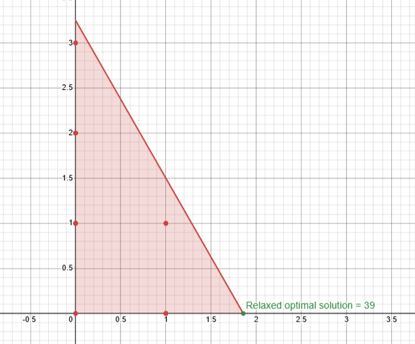
If we assume that the rounded solution in (1,0) that yields to a value of 21 is the optimal we would be wrong since:
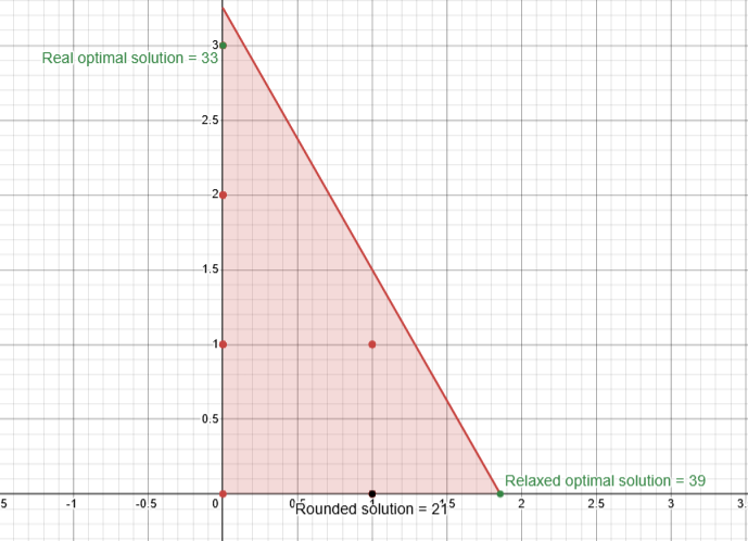
So what relation there is between the solution of the relaxation and the solution of the real one?
If we try to solve the problem through the graphical method we see that since the integrality constraint reduce the feasible area to a “lattice” , the relaxation is able to “follow” the gradient of the objective for longer yielding to a bigger value.
Formally:
For any ILP with max (min) , we have that z_{ILP} \leq z_{LP} (z_{ILP} \geq z_{LP}), i.e., the relaxation provides an upper bound (lower bound) on the optimal value of an ILP.
Transportation problem “pattern”
In the last section we implied that the solution of the relaxation is different from the original one and defines a bound for it.
There is an exception to this rule , where all vertexes of the feasible region lie on integer values (hence the two solutions are equal) , due to its correlation with a real life problem known as the “Transportation problem”, we’ll say that these problems have a Transportation problem pattern.
A problem in standard form:
\begin{align*} min \quad & \underline{c}^T \underline{x}\\ s.t.\quad & A\underline{x} \geq \underline{b}\\ \quad & \underline{x} = \underline{0} \quad \end{align*}
Has the transportation problem pattern if:
- \underline{b} is made of integers.
- A contains only either -1, 0 or 1.
- Each column has exactly K non-zero entries, where K = number of constraints families.
Now you may ask yourself , “what is a constraint family?”, this is a constraint family:
\sum_{j=1}^{n}{x_{ij}} \leq p_i, \quad i=1,\dots,m
So a collection of constraints that defines the same characteristic for different “elements” , in this case if this were the “plant capacity family” each member of this family describes the max capacity of each plant i to store n different types of elements.
Branch and Bound method

In the previous section we have seen that, in most cases, the optimal solution cannot be found directly through the linear relaxation of the problem, so we need a way to correct the relaxed solution into the real one, a possible way to do that is the Branch and Bound method.
But before talking about that we need to introduce two key concepts:
- Primal feasibility: all constraints are satisfied.
- Dual feasibility: all reduced costs have right signs.
What implications do these definitions have?
When we do a step in the primal simplex (normal simplex), we: 1. maintain primal feasibility. 2. improve dual feasibility.
We didn’t see yet how the dual simplex algorithm works, but we can say that it has the same effect as doing the primal simplex on the dual problem, what happens when we do that is: 1. we maintain dual feasibility. 2. we ‘repair’ primal feasibility (if broken).
We are going to use the dual simplex to keep the solution optimal and to make the new formulation feasible.
The method
We start by solving the linear relaxation of a problem:
\begin{align*} max \quad &z = 5 x_1 + 4x_2 \\ & x_1 + x_2 + x_3 = 5\\ & 10 x_1 + 6 x_2 + x_4 = 45\\ &x_1,x_2,x_3,x_4 \geq 0 \end{align*}
We solve it using primal simplex, and we reach the final tableau:
| x_1 | x_2 | x_3 | x_4 | ||
|---|---|---|---|---|---|
| -z | -\frac{95}{4} | 0 | 0 | -\frac{10}{4} | -\frac{1}{4} |
| x_2 | \frac{5}{4} | 0 | 1 | \frac{10}{4} | \frac{1}{4} |
| x_1 | \frac{15}{4} | 1 | 0 | -\frac{3}{2} | \frac{1}{4} |
The solution we found: \underline{x}^T=[\: \frac{15}{4} \quad \frac{5}{4} \quad 0 \quad 0 \: ] with value z = -\frac{95}{4} , is clearly not an “integer” one.
Here comes the Branch and Bound part:
We have two fractional value, we must choose one to start with, there are many techniques to do that , the most common one is to pick the bigger, but there aren’t wrong choices, you will eventually reach the solution choosing either of them.
We choose to branch on x_1 = 3.75 obtaining two new formulations:
flowchart TD
A(("(3.75,1.25,0,0)\n z=23.75"))
A -->|X1<=3| B((...))
A -->|X1=>4| C((...))
Starting from the left side, we now have a new constraints, the current solution is now unfeasible, if the graphical method is possible the solution can be trivially found, otherwise we would need tp redo the whole simplex again…..how annoying!!
There is another way, we can use the dual simplex:
In the dual simplex we apply the same rules as the primal, but we switch the roles of columns and rows:
First of all lets add the new constraint:
x_1 \leq 3
Let’s put it in normal form, by adding a new variable:
x_1 + x_5 = 3
Now let’s represent this constraint using non-basic variables , we will use the row of x_1:
x_1 - \frac{3}{2} x_3 + \frac{1}{4} x_4 = \frac{15}{4}
x_1 = \frac{15}{4} + \frac{3}{2} x_3 - \frac{1}{4} x_4
And we put it in our new constraint:
\frac{15}{4} +\frac{3}{2} x_3 - \frac{1}{4} x_4 + x_5 = 3
We get
\frac{3}{2} x_3 - \frac{1}{4} x_4 + x_5 = - \frac{3}{4}
And we add it to our tableau:
| x_1 | x_2 | x_3 | x_4 | x_5 | ||
|---|---|---|---|---|---|---|
| -z | -\frac{95}{4} | 0 | 0 | -\frac{10}{4} | -\frac{1}{4} | 0 |
| x_2 | \frac{5}{4} | 0 | 1 | \frac{10}{4} | \frac{1}{4} | 0 |
| x_1 | \frac{15}{4} | 1 | 0 | -\frac{3}{2} | \frac{1}{4} | 0 |
| x_5 | -\frac{3}{4} | 0 | 0 | \frac{3}{2} | -\frac{1}{4} | 1 |
Let’s now apply the dual simplex:
x_5 is the variable that will exit the basis, to choose the one that enter we look at the columns of that row, and we apply a min ratio test using the reduced costs and the value of the coefficients in that row, we got:
x_3: \frac{-\frac{10}{4}}{\frac{3}{2}} = -\frac{5}{3}
x_4: \frac{-\frac{1}{4}}{-\frac{1}{4}} = 1
In case of a minimization problem we multiply by -1 the ratio.
The variable x_4 will enter the basis, now we do a normal pivoting operation, and we got this tableau:
| x_1 | x_2 | x_3 | x_4 | x_5 | ||
|---|---|---|---|---|---|---|
| -z | -23 | 0 | 0 | -4 | 0 | -1 |
| x_2 | 2 | 0 | 1 | 1 | 0 | -1 |
| x_1 | 3 | 1 | 0 | 0 | 0 | 1 |
| x_4 | 3 | 0 | 0 | -6 | 1 | -4 |
We have reached a new optimal solution :\underline{x}^T=[\: 3 \quad 2 \quad 0 \quad 3 \quad 0 \: ] with value z = 23, this is a valid integer solution.
Even though this is a valid solution, we cannot be sure that is the best one.
How can we tell when the best solution is reached?
Now comes the bound part.
Lets update our diagram first:
flowchart TD
A(("(3.75,1.25,0,0)\n z=23.75"))
A -->|X1<=3| B(("(3,2,0,3,0)\n z=23"))
A -->|X1=>4| C((...))
We now explore the right side, doing the same operation we did before, and we get to a new solution:
flowchart TD
A(("(3.75,1.25,0,0)\n z=23.75"))
A -->|X1<=3| B(("(4,2,0,3,0)\n z=23"))
A -->|X1=>4| C(("(4,0.83)\n z=23.33"))
Clearly not an integer solution.
We keep going down that path:
flowchart TD
A(("(3.75,1.25)\n z=23.75"))
A -->|X1<=3| B((" (4, 2)\n z=23"))
A -->|X1=>4| C(("(4, 0.83)\n z=23.33"))
C -->|X2<=0| D(("(4.5, 0)\n z = 22.5"))
C -->|X2=>1| E(("..."))
We got a new non integer solution now if we compare its value with the integer one that we found, we see that it is smaller.
What does it mean?
We talked about how the relaxation provides an upper bound of the true solution, if we keep adding new constraints the bound that the relaxation provides get tighter, meaning that the more we branch the smaller the solution gets.
This means that all values that we would get by expanding that node are going to be less than or equal to 22.5, but we already got a valid solution of 23, so none of the values there interest us, we have bound that branch.
Let’s now see the right side:
We would like to enforce: x_2 \geq 1
Starting from the tableau of our previous solution:
| x_1 | x_2 | x_3 | x_4 | x_5 | ||
|---|---|---|---|---|---|---|
| -z | -\frac{70}{3} | 0 | 0 | 0 | -\frac{2}{3} | -\frac{5}{3} |
| x_2 | \frac{5}{6} | 0 | 1 | 0 | \frac{1}{6} | \frac{5}{3} |
| x_1 | 4 | 1 | 0 | 0 | 0 | -1 |
| x_3 | \frac{1}{6} | 0 | 0 | 1 | -\frac{1}{6} | -\frac{2}{3} |
So we build our new constraint:
x_2-x_6=1
We use the definition of x_2 in the tableau:
\frac{5}{6} - \frac{1}{6} x_4 -\frac{5}{3} x_5 -x_6 = 1
Put in normal form x_6:
\frac{1}{6}x_4 +\frac{5}{3}x_5 +x_6 = -\frac{1}{6}
Then we add it to the tableau:
| x_1 | x_2 | x_3 | x_4 | x_5 | x_6 | ||
|---|---|---|---|---|---|---|---|
| -z | -\frac{70}{3} | 0 | 0 | 0 | -\frac{2}{3} | -\frac{5}{3} | 0 |
| x_2 | \frac{5}{6} | 0 | 1 | 0 | \frac{1}{6} | \frac{5}{3} | 0 |
| x_1 | 4 | 1 | 0 | 0 | 0 | -1 | 0 |
| x_3 | \frac{1}{6} | 0 | 0 | 1 | -\frac{1}{6} | -\frac{2}{3} | 0 |
| x_6 | -\frac{1}{6} | 0 | 0 | 0 | \frac{1}{6} | \frac{5}{3} | 1 |
Two candidates for entering the basis, x_4 and x_5 but:
x_4: \frac{-\frac{2}{3}}{\frac{1}{6}} \leq 0
x_5: \frac{-\frac{5}{3}}{\frac{5}{3}} \leq 0
Min ratio test tells us that dual is unbounded, so the primal formulation is unfeasible.
flowchart TD
A(("(3.75,1.25)\n z=23.75"))
A -->|X1<=3| B((" (4, 2)\n z=23"))
A -->|X1=>4| C(("(4, 0.83)\n z=23.33"))
C -->|X2<=0| D(("(4.5, 0)\n z = 22.5"))
C -->|X2=>1| E((unfeasible))
And the solution is the one found in the first step.
Geometry of branch and bound
Let’s look at the previous problem under a geometrical point of view:
This is our original situation:
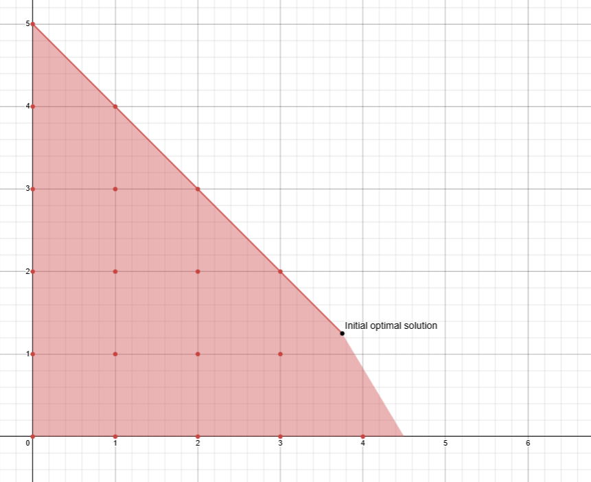
We split our problem in two section and found two new solutions:
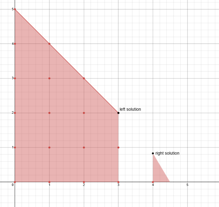
We kept the left one, and expanded the right section:
We found only one solution since the other formulation was unfeasible, amd we concluded that the first solution found was the best possible.
Cutting plane method

Another possible way to derive the integer solution from the relaxation, is through the Cutting planes method.
The idea is based upon this theorem:
For any feasible region X of an ILP, there exists an ideal formulation, but the number of constraints can be very large with respect to the size of the original formulation
What is this ideal formulation?
Basically a formulation where the boundaries of the feasible area lie on integer values, hence solving using simplex give the correct solution.
The concept might seem complicated, but is not so much different than the branch and bound method.
Instead of possibly cutting away large portions of the feasible area , we remove only the strict necessary, and to do that we use The Gomory fractional cuts.
Gomory fractional cuts

A Gomory fractional cut is a constraint that “cuts” away the decimal part of variable, specifically:
- Makes the current solution not feasible ( gets cut out).
- It’s satisfied by all integer feasible solutions.
But how do we derive a cut?
Let’s see it with an example:
Suppose that we want to find the cut corresponding to this constraint:
x_1-1.25x_2+0.25x_3 = 3.75
We expand the term as the sum of their lower bound and the remaining fractional part:
(1+0)x_1+(-2+0.75)x_2+(0+0.25)x_3 = (3+0.75)
Now we move all the integers to the right and all the decimal to the left:
0.75x_2 + 0.25x_3 - 0.75 = 3- x_1 + 2 x_2
Since on the right we have all integer , their sum must also be an integer, therefore the l.h.s. is also an integer:
\underbrace{0.75x_2 + 0.25x_3 - 0.75}_{integer} = \underbrace{3- x_1 + 2 x_2}_{integer}
Also, we can isolate the l.h.s. since the sum of the fractional parts is at least the fractional part of the sum (due to carries), and rewrite it like so:
0.75x_2 + 0.25x_3 - 0.75 \geq 0
That is equal to:
0.75x_2 + 0.25x_3 \geq 0.75
This is the Gomory cut of our constraint.
Back to the method
In order to find the integer solution we:
- Solve the relaxation.
- Pick the variable with the biggest fractional part.
- Create a cut and add it as a constraint.
- Fix the formulation with dual simplex.
- If the solution is reached we stop, otherwise back to step 2.
Let’s do an example:
We have a ILP in standard form:
\begin{align*} min \quad &z = -5 x_1-2 x_2 \\ s.t. \quad &2 x_1 +2 x_2 + x_3 = 5\\ & 2 x_1-2x_2+x_4 = 3\\ &x_1,x_2.x_3 \geq 0 , integers \end{align*}
We solve the Relaxation, and we get the final tableau:
| x_1 | x_2 | x_3 | x_4 | ||
|---|---|---|---|---|---|
| -z | 11 | 0 | 0 | \frac{7}{4} | \frac{3}{4} |
| x_2 | \frac{1}{2} | 0 | 1 | \frac{1}{4} | -\frac{1}{4} |
| x_1 | 2 | 1 | 0 | \frac{1}{4} | \frac{1}{4} |
We generate a cut for x_2:
\frac{1}{2} = x_2+ \frac{1}{4}x_3 -\frac{1}{4} x_4
\begin{align*} x_2(1 + 0) + x_3(0+0.25)+x_4(-1+0.75) & = (0 + 0.5)\\ 0.25 x_3 +0.75 x_4- 0.5 &= -x_2+x_4\\ 0.25 x_3+ 0.75 x_4 &\geq 0.5\\ 0.25 x_3+0.75 x_4 -x_5 &= 0.5\\ x_5 - 0.25 x_3 -0.75 x_4 &= -0.5 \quad (1) \end{align*} We add (1) to the tableau:
| x_1 | x_2 | x_3 | x_4 | x_5 | ||
|---|---|---|---|---|---|---|
| -z | 11 | 0 | 0 | \frac{7}{4} | \frac{3}{4} | 0 |
| x_2 | \frac{1}{2} | 0 | 1 | \frac{1}{4} | -\frac{1}{4} | 0 |
| x_1 | 2 | 1 | 0 | \frac{1}{4} | \frac{1}{4} | 0 |
| x_5 | -\frac{1}{2} | 0 | 0 | -\frac{1}{4} | -\frac{3}{4} | 1 |
Two candidates are available x_3 and x_4, lets check the ratios:
x_3: -1 \times \frac{7/4}{-1/4} = 7
x_4: -1 \times \frac{3/4}{-3/4} = 1
The variable x_4 will enter the basis, after pivoting we got:
| x_1 | x_2 | x_3 | x_4 | x_5 | ||
|---|---|---|---|---|---|---|
| -z | \frac{21}{2} | 0 | 0 | \frac{3}{2} | 0 | 1 |
| x_2 | \frac{2}{3} | 0 | 1 | \frac{1}{3} | 0 | -\frac{1}{3} |
| x_1 | \frac{11}{6} | 1 | 0 | \frac{1}{6} | 0 | \frac{1}{3} |
| x_4 | \frac{2}{3} | 0 | 0 | \frac{1}{3} | 1 | -\frac{4}{3} |
Still no integer solution, the biggest fractional part is of x_1, so we generate a new cut:
x_6-\frac{1}{6}x_3-\frac{1}{3}x_5 = -\frac{5}{6}
We add it to the tableau and perform a step of the dual simplex, we end up with:
| x_1 | x_2 | x_3 | x_4 | x_5 | x_6 | ||
|---|---|---|---|---|---|---|---|
| -z | 8 | 0 | 0 | 1 | 0 | 0 | 3 |
| x_2 | \frac{3}{2} | 0 | 1 | \frac{1}{2} | 0 | 0 | -1 |
| x_1 | 1 | 1 | 0 | 0 | 0 | 0 | 1 |
| x_4 | 4 | 0 | 0 | 1 | 1 | 0 | -4 |
| x_5 | \frac{5}{2} | 0 | 0 | \frac{1}{2} | 0 | 1 | -3 |
Still no integer solution , we cut again , the biggest fractional is that of x_5 , we generate a new cut:
x_7-\frac{1}{2}x_3 = -\frac{1}{2}
We perform the usual steps, and we got this tableau:
| x_1 | x_2 | x_3 | x_4 | x_5 | x_6 | x_7 | ||
|---|---|---|---|---|---|---|---|---|
| -z | 7 | 0 | 0 | 0 | 0 | 0 | 3 | 2 |
| x_2 | 1 | 0 | 1 | 0 | 0 | 0 | -1 | 1 |
| x_1 | 1 | 1 | 0 | 0 | 0 | 0 | 1 | 0 |
| x_4 | 3 | 0 | 0 | 0 | 1 | 0 | -4 | 2 |
| x_5 | 2 | 0 | 0 | 0 | 0 | 1 | -3 | 1 |
| x_3 | 1 | 0 | 0 | 1 | 0 | 0 | 0 | -2 |
We got our integer solution, we can stop here.